Neural activity sonification: a step-by-step creative workflow
Your neural activity sonification project can fail before the first sound reaches the speakers. The usual culprit is not the synthesizer, the room, or even the fish.
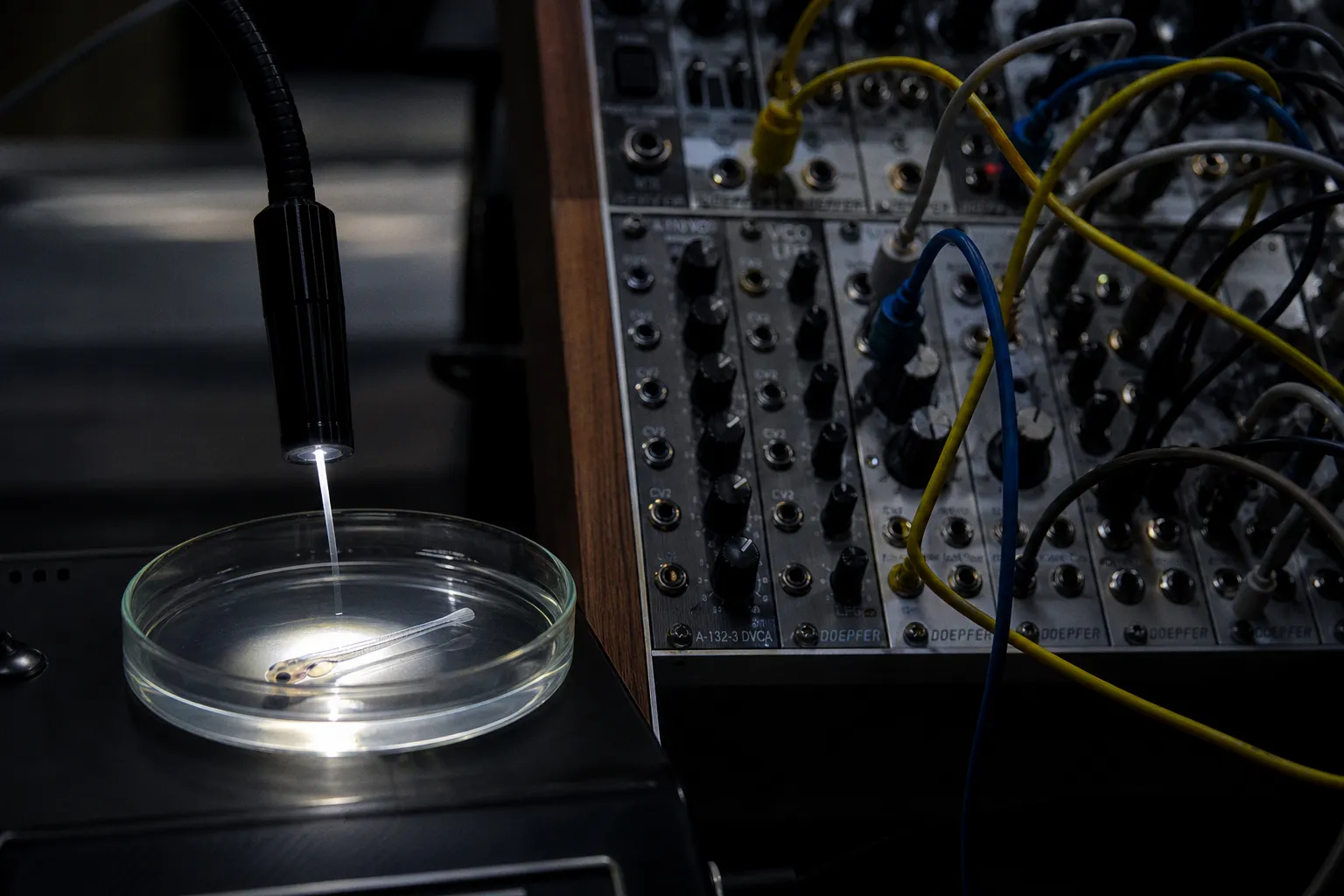
It is the data pipeline: a noisy trace gets cleaned too aggressively, spike timing gets rounded, or three unrelated variables are mapped to pitch until the final piece sounds busy rather than informative.
Let’s fix that at the bench, where these projects actually live. Converting brain data to sound is not a matter of pressing “play” on an EEG recording and waiting for the brain to compose a charming little concerto. Neural signals need a clear question, careful preprocessing, an explicit mapping strategy, and enough restraint to let meaningful changes survive the trip from electrode or microscope to loudspeaker.
The most useful way to think about neural activity sonification project steps is as a chain:
1. acquire and document the neural signal;
2. remove technical noise without erasing biology;
3. decide what the listener should hear;
4. map neural variables to sound;
5. synthesize and spatialize the result;
6. validate the audio against the original data;
7. only then design the exhibition, performance, or public-facing piece.
That order matters. A beautiful soundscape built on an opaque mapping is still opaque. We can make the work expressive without pretending that the data naturally contain a hidden melody.
Start with the biological question, not the instrument
Before choosing a scale, a drone, or a wonderfully expensive multichannel speaker system, write one sentence describing what the audience should be able to notice.
For a zebrafish project, that sentence might be:
- listeners should hear how neural activity changes between two behavioral states;
- the installation should make local differences across brain regions perceptible;
- the piece should preserve the irregular timing of discrete neural events;
- the audience should compare spontaneous activity with activity during a stimulus.
Each goal points toward a different workflow. If you want to communicate broad changes in network state, frequency-band power or activity envelopes may be useful. If the timing of individual events matters, you need an event-based representation. If spatial organization is central, electrode or imaging coordinates should influence the placement of sound rather than merely decorate the visual layer.
This is the first place where projects often wander off. Someone sees a clean trace, maps it to pitch, adds reverb, and discovers that every condition sounds almost identical. The mapping has produced audio, but not a clean signal.
The listener cannot hear your biological question unless you make that question control something in the sound.
Document the acquisition context at the beginning: species and preparation, recording modality, sampling rate, channel or region labels, behavioral condition, stimulus timing, missing segments, and any preprocessing already performed. For zebrafish neural activity, keep the anatomical reference especially clear. A channel label such as “left optic region” or “dorsal cluster” is much more useful later than an anonymous column called channel_07.
You do not need to expose every technical detail in the final exhibition. You do need to preserve them in the working files. Art audiences deserve a coherent experience; your future self deserves not to reverse-engineer the entire project from a mysterious audio render named final_final_2.wav.
Choose the sonification method that matches the signal
There are three useful families of neural data sonification. They are related, but they do different jobs.
Direct audification: let the waveform become the starting material
In direct audification, the recorded signal is routed into an audio system or converted into an audible range with minimal transformation. The historical roots of this approach reach back to 1934, when Edgar Adrian and Brian Matthews routed analogue EEG signals to an audio amplifier.
This method can preserve the texture of a recording, including irregularity and temporal detail. It is attractive when the raw signal itself has a strong character or when the project asks what neural activity sounds like before artistic intervention.
The catch is that neural signals often sit outside the range or timescale that makes sense for human hearing. A slow signal may need time compression; a high-frequency recording may need scaling or filtering. Once you shift the time or frequency axis, you are no longer offering an untouched acoustic translation. You are making a perceptual adaptation, which is perfectly reasonable—as long as you describe it clearly.
Direct audification works well when:
- the audience should encounter the continuous texture of the signal;
- you want minimal interpretive mapping;
- the project can tolerate a less traditionally musical result;
- the raw trace has already passed careful artifact control.
It works less well when several channels overlap into an undifferentiated wash. If everything goes straight to the same stereo pair, the audience may hear density but not structure.
Parameter-mapped sonification: assign neural variables to sound properties
Parameter-mapped sonification, or PMS, maps selected neural variables to sound attributes such as pitch, amplitude, timbre, duration, or spatial location.
For example, you might map:
- alpha-band power to a slowly changing filter;
- low-beta power to brightness or harmonic content;
- high-beta power to a short layer of increased density;
- spike rate to event frequency;
- the location of a channel or region to speaker position;
- stimulus onset to a change in synthesis mode rather than a loud accent.
This is usually the most approachable method for public engagement because you can explain the relationship in a sentence. The audience does not need to understand every detail of electrophysiology to grasp that one feature of the sound tracks one feature of the data.
But PMS can become a mapping junk drawer. Pitch, volume, panning, distortion, duration, and tempo all changing at once may feel sophisticated in the patch and incoherent in the gallery. Start with one or two mappings. Add another only when the first pair has become interpretable.
A practical mapping table might look like this:
| Neural variable | Sound parameter | Why it helps | Main risk |
|---|---|---|---|
| Band power over time | Filter brightness or harmonic richness | Preserves gradual state changes without forcing a melody | Slow trends can become visually or sonically dull |
| Spike timing | Short percussive event | Keeps discrete events perceptible | High event density can turn into clicks or noise |
| Spike rate in a time window | Event density or note repetition | Makes activity level easy to compare | Rate hides the exact timing of individual events |
| Channel or brain-region position | Spatial speaker location | Connects anatomy with the listening space | Poor calibration can make spatial meaning arbitrary |
| Signal amplitude envelope | Loudness within a narrow range | Intuitive for broad fluctuations | Amplitude artifacts may become dramatic but misleading |
Notice the phrase “within a narrow range.” If raw amplitude controls loudness with no normalization, one large artifact can dominate the whole piece. A mapping should make the intended biological variation audible, not reward the worst cable movement of the afternoon.
Model-based sonification: let the data drive a dynamic system
Model-based sonification, or MBS, places a dynamic model between the data and the sound. The data configure the model, and the model produces sound when excited.
A useful MBS design considers six components:
1. setup;
2. dynamics;
3. excitation;
4. initial state;
5. link variables;
6. listener characteristics.
This approach is more interpretive than direct audification and usually more conceptually demanding than PMS. It can be powerful for installations because the listener hears a responsive system rather than a literal transcription of a trace. Neural variables might alter the tension, damping, resonance, or movement of a virtual object.
The discipline here is to explain the model. If neural activity controls a simulated resonant body, tell the audience what changes and what remains fixed. Otherwise, the sound may be compelling while the scientific relationship disappears behind the metaphor.
For a first project, PMS is often the most manageable entry point. Direct audification is useful when signal texture is the subject. MBS becomes especially interesting when you want the artwork to explore emergence, interaction, or the behavior of a neural system rather than simply report a measurement.
Build the data pipeline before you build the composition
The neuroscience data sonification workflow should have a plain, inspectable intermediate stage. Before generating musical material, create a cleaned dataset containing the variables you intend to sonify and nothing you cannot explain.
1. Preserve the raw recording
Keep the raw files read-only. Make a separate working copy for filtering, alignment, normalization, and feature extraction. Record every transformation with enough detail to reproduce it later.
For imaging data, that may include motion correction, segmentation, baseline correction, and extraction of activity traces. For electrophysiology, it may include filtering, artifact rejection, channel selection, and spike detection. The exact operations depend on the modality, but the principle stays the same: do not bury preprocessing inside an audio patch where nobody can see what happened.
2. Identify noise that is technical, not biological
Noise is not simply “anything irregular.” Neural activity is often irregular. A perfectly smooth trace may be a sign that you have removed the interesting part.
Look for:
- mains interference and electrical hum;
- movement artifacts;
- saturation or clipped recordings;
- stimulus markers that drift relative to the neural signal;
- missing samples;
- unstable channels;
- fluorescence changes caused by motion rather than neural activity;
- discontinuities introduced by file concatenation.
Use visual inspection alongside automated measures. A filter can remove a known interference band, but it cannot decide whether a sudden change is a genuine event or a loose connection. That requires context.
If your audience will hear a large change, you should be able to point to the corresponding feature in the processed data and explain why you kept it.
3. Align neural events with behavior and stimulus timing
A zebrafish neural activity audio piece becomes much more informative when its sound can be related to something else: movement, sensory stimulation, social interaction, or a change in experimental condition.
Align the timelines before mapping. If stimulus onset arrives late in the audio because of a timestamp mismatch, the artwork may communicate a false causal relationship. The audience will not see the timestamp error; they will simply hear a convincing story that the data do not support.
4. Decide whether your unit is a trace, a window, or an event
This decision determines the entire sound design.
- A continuous trace supports evolving textures, filters, amplitude envelopes, and slow spatial movement.
- A time window supports summaries such as mean power, variance, event count, or band ratios.
- A discrete event supports clicks, plucks, grains, short notes, or triggers.
Do not use event counts when exact timing is the scientific point. Conversely, do not send every detected event directly to a speaker when the event rate is so high that individual events become inaudible.
Preprocessing should remove technical noise, not remove the uncomfortable irregularity that makes neural data neural.
Map the signal without pretending it is already music
The most common artistic shortcut is to map a neural variable directly to a musical scale and then describe the result as the brain “playing” the composition. That framing is tempting, but it overstates what the data provide.
Neural activity does not naturally compose pleasant tonal music. The pleasantness comes from your mapping rules, pitch quantization, synthesis choices, rhythmic constraints, and mixing decisions. That is not a weakness. It is the creative and analytical work of the project.
Start by defining the mapping range. Suppose a normalized feature varies between 0 and 1. You might map it to a controlled filter cutoff, a modest amplitude range, or a selected group of pitches. Keep the output range narrow enough that the audience can detect change without being overwhelmed.
Then test the mapping with deliberately simple cases:
- constant input;
- slowly rising input;
- alternating high and low input;
- sparse events;
- dense events;
- a known artifact;
- a real segment from each experimental condition.
These tests reveal whether your mapping behaves as intended. If a constant input produces a drifting sound, the synthesis system is adding movement that does not come from the data. If a single artifact creates a theatrical explosion, the scaling needs attention.
What if the recording contains irregular spike timing?
Preserve it. When mapping neural spikes to audio or MIDI, timing precision matters. Some MIDI-generation workflows round note times to a 1/16-note grid, which can erase the very temporal differences you want the listener to hear.
In Python, packages such as music21 can be preferable for discrete spike-to-MIDI workflows where you need more control over irregular event timing. Still, inspect the resulting file rather than trusting the library. Exported MIDI may pass through additional quantization or DAW settings that quietly tidy the timing.
If the precise timing is too dense for direct listening, create two layers:
- an event layer that preserves timing but uses a restrained, granular texture;
- a slower summary layer that communicates overall activity level.
That gives the listener both the nervous detail and the broader shape.
What if several neural features produce conflicting sound changes?
Reduce the number of active controls. Let one feature control pitch or spectral position, another control event density, and keep loudness mostly stable. If every variable controls loudness, the piece becomes a volume meter with ambitions.
A good mapping should also be reversible enough for you to reason about. You do not need the audience to reconstruct the original trace by ear, but you should be able to explain whether a brighter sound means more activity, higher frequency-band power, a change in region, or simply a compositional transition.
Keep the signal audible in the room
A sonification can be scientifically careful and still fail as an installation. The gallery is not a headphone edit suite. People enter midway through the piece, talk over it, stand in different positions, and listen for much shorter periods than you expect.
Use spatialization only when it carries meaning
In a three-dimensional EEG audio installation, speaker placement can correspond to electrode positions on the scalp. Frontal signals can trigger front speakers, lateral or medial signals can control middle speakers, and occipital signals can drive rear speakers.
That structure is useful when spatial anatomy is part of the concept. It is not useful when every channel is panned randomly because the room has eight speakers and someone wants all eight to work.
Calibrate the system with a simple test signal for each channel. Confirm that the front channel sounds front, the rear channel sounds rear, and that the mapping still makes sense from the places where visitors actually stand. A spatial design that only works from one taped X on the floor is an installation puzzle, not an accessible artwork.
Separate analysis, routing, and synthesis
Real-time projects often route data between an analysis environment and a sound system using Open Sound Control, or OSC. Tools such as SuperCollider, Max/MSP, and Ableton Live can receive and transform these messages.
SuperCollider’s default incoming OSC port is 57120, but port numbers are only one small part of the setup. You also need stable message names, consistent value ranges, timestamps or sensible buffering, and a clear response to missing data.
For example, decide what happens if the neural stream pauses:
- does the sound hold its last value?
- does it fade to a neutral state?
- does the system switch to a pre-recorded segment?
- does the installation announce a technical problem?
A silent failure is especially dangerous in a public artwork because visitors may interpret it as part of the piece. Sometimes that is charming. Usually it is a network cable having a private joke at your expense.
Build a rendered version before committing to real time
Real-time neural sonification is attractive because it promises liveness, but it also introduces latency, dropouts, clock drift, and unstable behavior. Produce an offline render first. Compare it with the live system using the same input segment.
If the live version sounds different, identify why. Is the difference caused by buffering, feature-window size, OSC routing, synthesis load, or a deliberate change in the mapping? Do not call every technical artifact “emergence.”
For public engagement, a hybrid system is often stronger: the installation can use live or near-live data for one layer while a stable, pre-rendered structure preserves continuity and intelligibility.
Validate the artwork as both experiment and communication
Validation does not mean asking whether the piece sounds nice. It means asking whether the sound does what you claim.
Run at least three kinds of checks.
Data-to-sound checks
Play synthetic test inputs and confirm that each mapping responds correctly. Test the minimum, midpoint, and maximum of every control. Test missing values and sudden outliers. Save short audio examples so you can compare revisions without relying on memory.
Sound-to-data checks
Take a recognizable audio event and trace it backward. Which neural feature caused it? Which transformation changed its timing or intensity? If you cannot answer, the pipeline has become too opaque.
Audience checks
Ask listeners what they think they are hearing, but do not quietly reward the answer you hoped for. If someone assumes that a low pitch means low neural activity, and your mapping actually uses low pitch for frontal position, the interpretive design needs work.
Labels can help. A concise wall text might state that the piece maps event timing to percussive triggers and regional activity to spatial position, while a changing filter represents a selected frequency-band measure. That gives visitors a key without turning the exhibition into a methods supplement.
Avoid claims that the audio reveals a single true sound of the brain or that one musical pattern corresponds universally to one cell type. No standardized musical mapping scale exists for specific cell types across sci-art projects. Every mapping is a designed translation with assumptions.
A practical production sequence
Once the conceptual and technical decisions are clear, the work can move in a reliable order:
1. Create a data dictionary. Define every channel, region, feature, unit, timestamp, and missing-value rule.
2. Make a clean analysis file. Keep raw and processed data separate, and log each preprocessing operation.
3. Extract a small feature set. Begin with one continuous measure and one event-based measure rather than sonifying everything.
4. Prototype with neutral sounds. Use simple tones, clicks, noise bands, or short grains before composing a polished palette.
5. Test edge cases. Feed the system constant, sparse, dense, extreme, and missing inputs.
6. Render short comparison studies. Create versions for each condition and listen side by side.
7. Add spatial or visual layers. Only after the core mapping communicates clearly in a simple playback setup.
8. Stress-test the live system. Check latency, dropped messages, reconnect behavior, CPU load, and audio output levels.
9. Prepare an audience explanation. State what the data are, what the sound controls mean, and where artistic transformation begins.
10. Archive the project. Save raw data references, processed files, mapping notes, software versions, renders, and installation settings.
The order is deliberately unglamorous. That is a compliment. Reliable sci-art usually depends on a great deal of preparation that the audience should never have to notice.
Where the creative work becomes visible
Once the pipeline is stable, you can make compositional choices with confidence. You can choose whether a spike becomes a dry click or a resonant grain, whether a change in band power opens a filter or shifts a harmonic field, and whether different neural regions occupy distinct acoustic spaces.
You can also decide how much information to expose. A public installation does not need to sonify every sample. It may be more honest to slow the activity down, isolate a meaningful episode, or combine a continuous neural texture with a readable event layer. The piece can be less literal and more understandable at the same time.
The key is to label the transformations. Time compression, normalization, filtering, pitch quantization, event aggregation, and spatial mapping all shape what the audience hears. Naming them does not drain the magic from the work. It tells the audience where the science ends, where the design begins, and how carefully the bridge between them was built.
Neural activity sonification is strongest when the audio preserves a real relationship to the data while admitting that listening is an authored experience. We are not uncovering a secret song hidden inside a zebrafish brain. We are designing a way for neural dynamics to become perceptible through sound—with all the precision, compromise, and occasional cable-related nonsense that serious lab work requires.
So start small. Pick one question, one clean signal, and one mapping you can explain without waving your hands. Run the edge-case tests. Listen for noise that is really a preprocessing mistake, and for smoothness that has erased the biology. Then add the artistic layer deliberately.
That is how you get from raw neural activity to a soundscape that is not only engaging, but trustworthy enough to stand beside the data.