Neural data to MIDI: fast audio conversion for sci-art
Neural data does not arrive in a form that music can immediately understand. An EEG trace is a changing voltage measured at the scalp; calcium imaging records fluorescence across cells; a zebrafish…
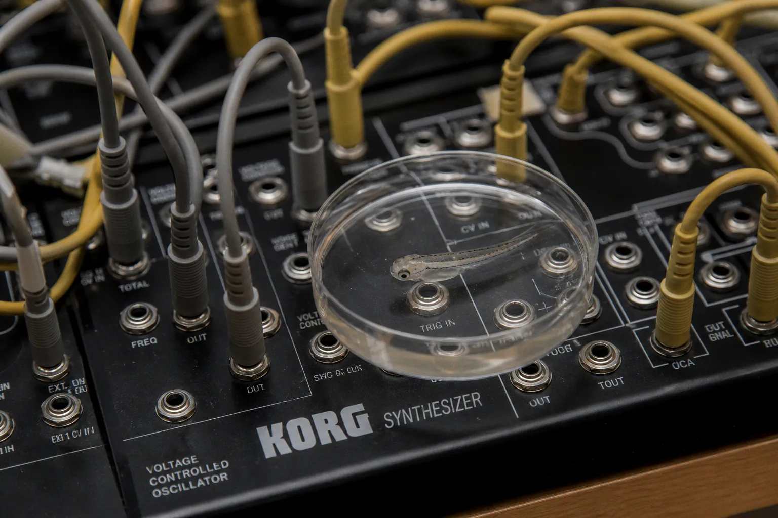
Neural data does not arrive in a form that music can immediately understand. An EEG trace is a changing voltage measured at the scalp; calcium imaging records fluorescence across cells; a zebrafish brain may contain tens of thousands of active neurons distributed through a small, transparent body. To turn any of this into MIDI, the researcher must decide what each biological feature will become: pitch, velocity, duration, timbre, spatial position, or control data.
That decision is the real instrument. MIDI is only the message layer.
A successful neural data to MIDI conversion therefore does not attempt to make the brain “play music” without mediation. It builds a controlled relationship between neuronal activity and musical parameters. The clearest systems preserve a traceable link to the biology while giving the listener enough contrast, rhythm, and luminance-like separation to perceive change. Without that structure, the result is often an undifferentiated stream of notes: technically active, perceptually empty.
Translating neuronal spikes into musical parameters
The most direct mapping treats neuronal activity as an event stream. A spike, threshold crossing, or increase in fluorescence can trigger a MIDI note. The strength of the event can control velocity. Its location in the brain can determine pitch or instrument. Time remains time, although it may be compressed, expanded, or quantized for performance.
A useful first translation looks like this:
| Neural feature | MIDI or musical parameter | Perceptual effect |
|---|---|---|
| Spike or activity threshold crossing | Note-on event | Makes individual neuronal events audible |
| Firing rate or fluorescence intensity | Note velocity | Produces louder or softer attacks |
| Neuron position along an anatomical axis | Pitch | Turns spatial organization into melodic contour |
| Activity duration | Note length or sustain | Reveals persistence rather than isolated events |
| Frequency band in EEG | Instrument, register, or MIDI channel | Separates slow and fast oscillatory activity |
| Left/right hemisphere activity | Tuning, stereo position, or paired instruments | Makes lateralized behavior easier to hear |
| Region of interest | Instrument assignment or timbral layer | Preserves anatomical grouping |
The mapping should be chosen according to the question being asked. If the purpose is exploratory analysis, a transparent one-to-one relationship is often preferable. If the purpose is public performance, some compression and orchestration may be necessary. Those are different objectives, and confusing them produces weak science communication.
The Brain Orchestra, a collaborative project by Sébastien Wolf and Vincent Goudard, approaches this problem by loading datasets as binary matrices and translating them into MIDI messages. In that system, note velocity is mapped to neuronal activity. The result retains a visible computational pathway: data enter as structured states, and the musical output changes as those states change.
This kind of architecture is valuable because it leaves room for inspection. A listener may hear a dense passage, but the researcher can still return to the underlying matrix and ask which rows, columns, or activity values generated it. The sound is not merely inspired by neuroscience. It is indexed to a dataset.
MIDI does not carry meaning by itself; meaning appears when the mapping between biology and sound remains legible.
For a first neural data sonification tool, begin with a narrow parameter set. Map only two or three variables and listen for whether they remain distinguishable. A practical starting configuration might use time for note onset, activity amplitude for velocity, and anatomical position for pitch. Adding timbre, panning, modulation, and multiple scales too early can increase cognitive load faster than it increases information.
Preserve the shape of the signal
Neural recordings are rarely ready for direct conversion. They may contain missing frames, motion artifacts, baseline drift, inconsistent sampling intervals, or far more channels than a listener can separate. Preprocessing should reduce these problems without erasing the behavior that the sonification is meant to reveal.
A compact preparation sequence is:
1. Define the biological unit. Decide whether the event is a spike, a frame-level fluorescence value, a frequency-band amplitude, or a region-level average.
2. Normalize within the dataset. Relative activity is usually more useful than raw intensity when recordings vary between animals or sessions.
3. Set an activity threshold. This prevents low-level noise from triggering a continuous cloud of MIDI events.
4. Reduce the channel count deliberately. Grouping by anatomical region, behavior, or functional cluster is often more perceptually meaningful than arbitrary downsampling.
5. Map the remaining values to bounded musical ranges. For example, constrain velocity to a usable MIDI interval and pitch to a defined scale.
6. Keep a record of every transformation. A performance patch should be reproducible enough that another researcher can reconstruct its logic.
The final point is easy to neglect. A visually elegant interface can conceal an unstable mapping. If normalization changes between sessions, a louder passage may represent stronger neuronal activity—or simply a different scaling choice. The audience does not need to see every line of preprocessing, but the scientific team must know where interpretation ends and aesthetic intervention begins.
Mapping zebrafish calcium imaging to FM synthesis
Calcium imaging offers a particularly rich source for sound because fluorescence values vary across many cells and frames. In larval zebrafish, light-sheet microscopy can capture activity across a large portion of the nervous system while the animal develops and responds to stimuli. The resulting data are spatially dense, temporally complex, and visually compelling. They also require care: a fluorescence trace is not identical to an instantaneous action potential.
One sonification tool presented at SMC 2020 used manually drawn Regions of Interest, or ROIs, in zebrafish calcium imaging. The average fluorescent values of those regions were mapped to parameters of FM synthesis. This is a useful design choice because FM synthesis can expose gradual changes in a signal through evolving brightness and sidebands, rather than relying only on discrete note events.
In an FM synthesizer, a carrier oscillator is shaped by a modulator. Changing the modulation index can make a tone more complex and spectrally bright; changing frequency can move the sound through register or timbre. For calcium imaging, this creates several plausible mappings:
- Average fluorescence controls modulation depth, producing a brighter or more intricate tone as activity rises.
- ROI identity selects the carrier register or instrument layer.
- Temporal derivative—the speed of fluorescence change—controls attack sharpness or modulation rate.
- Spatial position determines stereo placement or a slow pitch offset.
- Separate anatomical regions occupy distinct MIDI channels.
The important distinction is between absolute level and change. A cell can remain highly active without generating a new event, while a rapid rise in fluorescence may be biologically meaningful even if the absolute value remains moderate. A sonification that maps only the instantaneous value may flatten these differences. A second layer based on the rate of change can restore them.
Converting calcium imaging to sound without creating noise
Calcium imaging often has a slower temporal profile than electrophysiological recordings. If every frame becomes a note, the output can feel like a machine reading a spreadsheet aloud. A better approach is to separate continuous and event-based information.
Continuous fluorescence can drive synthesis parameters such as:
- modulation depth;
- filter cutoff;
- amplitude envelope;
- spatial panning;
- harmonic density.
Discrete events can be generated from:
- threshold crossings;
- local maxima;
- onset of a synchronized ROI response;
- transitions between behavioral states.
This two-layer structure keeps the sonic surface readable. The continuous layer describes the field of activity; the event layer marks changes that deserve attention.
The choice of ROI also carries scientific meaning. Manually drawn regions are not neutral containers. They reflect the researcher’s anatomical question, segmentation practice, and interpretation of the image. If a region covers several functionally distinct structures, its average may produce a smooth but misleading value. If the ROIs are too small, the sonification may become unstable and overly granular.
A practical workflow is to begin with four to eight ROIs, assign each a restrained frequency range, and listen before adding more. The brain contains more information than a loudspeaker can present simultaneously. Reduction is not a failure of fidelity; it is the condition that allows a pattern to remain perceptible.
Spatial and temporal mapping in a zebrafish brain
A neural recording is not only a timeline. It is also an arrangement of cells, regions, pathways, and asymmetries. Spatial mapping can reveal an organization that is difficult to see in a dense image, especially when thousands of neurons change together.
In one granular synthesis sonification of a zebrafish larva’s brain, a dataset containing 23,743 neurons recorded with light-sheet microscopy was downsampled to 8,000 points. The pitch was mapped to neuronal position along the spinal cord axis across four octaves of a diatonic scale.
This is a decisive aesthetic and analytical choice. The listener does not hear 23,743 independent voices. Instead, the dataset is reduced to a playable density while preserving a spatial gradient. A neuron’s position becomes a pitch coordinate, and the four-octave range gives the anatomical axis enough room to form a contour.
Granular synthesis is well suited to this kind of data because it works with short sound grains rather than conventional notes. Each grain can inherit a location, amplitude, duration, or spectral quality from a data point. When many grains overlap, the result may resemble a cloud, texture, or field of particles. This is closer to the structure of a neural population than a traditional melody is.
Yet granularity must be controlled. If every point receives identical duration and amplitude, spatial organization disappears into texture. Introduce contrast through a small number of stable rules:
1. Use pitch for one anatomical axis, not several at once.
2. Reserve velocity for activity strength so that loudness retains a clear interpretation.
3. Let grain density reflect event frequency or population synchrony.
4. Use a fixed scale to prevent small numerical fluctuations from becoming distracting microtonal noise.
5. Keep the downsampling method documented, particularly when selecting thousands of points from a larger population.
A diatonic scale across four octaves is not biologically “natural,” but it gives the ear a coherent coordinate system. The scale acts like a visual palette: it limits the number of competing hues so that movement can be seen—or, in this case, heard.
A spatial sonification should make anatomy feel organized, not merely make the dataset feel large.
Lateralized activity and behavior
The larval zebrafish offers a clear example of how neural asymmetry can become an audible behavioral cue. Activity in the Anterior Rhombencephalic Turning Region, or ARTR, correlates with leftward and rightward swimming movements. Sonifying the two hemispheres with different musical tunings allows the alternation of activity to become audible.
This mapping is stronger than simply assigning the left side to a low note and the right side to a high note. Different tunings can create a perceptual tension between two systems. When one hemisphere dominates, one tonal character becomes more present; when activity shifts, the balance changes. The listener can follow the alternation without needing a screen.
The same principle applies to other paired regions. Use stereo placement when spatial opposition is central. Use contrasting timbres when the output will be heard on speakers in a gallery. Use separate MIDI channels when the performance system needs independent control. The parameter should serve the anatomy, not decorate it.
The habenula provides a contrasting case. In a dataset of a few hundred zebrafish neurons, activity showed asynchronous peaks: neurons fired in sequences rather than simultaneously. The resulting sonification resembled a monodic melody instead of harmonic chords. This is an important reminder that musical form can emerge from the temporal relationship between cells.
If neurons activate together, chords or dense clusters may be appropriate. If they activate in sequence, a melodic line may reveal the organization more clearly. The sound should follow the structure of the data, even when the result is less spectacular than a full-spectrum wash.
Real-time EEG sonification: from Muse to DAW
Calcium imaging usually belongs to a laboratory or post-processing workflow. EEG offers a more immediate route from neural activity to sound. A wearable headband can stream signals while a performer, participant, or researcher interacts with a digital audio workstation. But real-time does not mean direct. EEG bands are statistical summaries of electrical activity, not readable channels for thoughts or emotions.
A brain wave MIDI generator typically maps frequency bands to musical controls. MindMIDI, a free real-time brainwave sonification software, routes spectrum bands such as Delta/Theta, Alpha, and Beta/Gamma to different instruments, including cello, piano, and violin, within a DAW. Brain2MIDI, an Android application, converts brainwaves from a Muse headband into MIDI notes and Control Change signals, transmitting them through USB, Wi-Fi, or Bluetooth to synthesizers or VJ software.
These systems are most useful when their mappings are treated as control surfaces. An increase in an alpha-band measure might raise a filter cutoff or alter the balance of an instrument. It does not mean that the software has isolated a single mental state and translated it into a complete composition. The mapping is a designed interpretation of a signal.
For an EEG-to-MIDI performance, separate the musical system into three layers:
- Signal layer: acquisition, filtering, artifact rejection, and band-power calculation.
- Mapping layer: rules that convert normalized features into notes, velocity, pitch, or CC messages.
- Musical layer: instruments, effects, scales, tempo, looping, and performance constraints.
Keeping these layers distinct makes the setup easier to debug. If the output becomes erratic, the researcher can ask whether the instability began in the EEG signal, the mapping function, or the synthesizer patch. A single large patch hides the source of the problem behind its surface complexity.
BrainAccess MIDI illustrates a more research-oriented option. It is a commercial 16-channel wireless EEG device intended for research, education, and development rather than medical diagnosis. The kit streams EEG data over Bluetooth, and its specifications include a 250 Hz sampling rate for cognitive tasks. Its listed price is €1,600 excluding VAT, which places it in a different category from a hobbyist headband or a software-only experiment.
The choice of hardware should follow the intended output:
| Use case | Suitable approach | Main compromise |
|---|---|---|
| Classroom demonstration | Consumer headband with a simple MIDI app | Limited signal quality and fewer channels |
| Live audiovisual performance | Muse plus Brain2MIDI or a comparable bridge | Convenience may outweigh physiological detail |
| Controlled cognitive experiment | Multi-channel research EEG such as BrainAccess MIDI | Higher cost and greater setup demands |
| Zebrafish laboratory study | Calcium imaging pipeline with ROI-based mapping | Requires imaging access and careful preprocessing |
| Dataset-based exhibition | Offline MIDI rendering from recorded neural data | Less immediacy, but greater reproducibility |
A reliable performance also needs an audible fallback. Bluetooth interruptions, dropped packets, electrode impedance changes, and movement artifacts are ordinary engineering problems. The audience should hear a stable musical environment even if the incoming signal momentarily disappears. Hold the last valid value, fade into a controlled texture, or switch to a documented baseline state. Silence can be meaningful, but accidental silence usually reads as a broken installation.
Building a repeatable neural data sonification workflow
The strongest projects move between visual and auditory inspection. A plot may reveal a slow drift that the ear interprets as a changing timbre. A sound may expose a repeated temporal motif that is difficult to notice in a crowded heatmap. Neither medium replaces the other.
A practical workflow for neural data to MIDI conversion can be organized as follows.
1. Start with a biological question
Do you want to hear synchrony, lateralization, spatial position, oscillation, or behavioral transitions? If the question is not defined, the mapping will tend to accumulate parameters until the output becomes impressive but uninterpretable.
For example, if the question concerns left/right swimming, begin with paired activity traces from the ARTR. If it concerns spatial organization, retain neuron coordinates and avoid reducing everything to a single global amplitude.
2. Choose the smallest useful dataset
A full recording may contain more channels than the final work needs. Select a time window, region, or behavioral episode. For calcium imaging, ROI averages may be sufficient. For a large population dataset, use a principled downsampling strategy rather than selecting points because they sound interesting.
3. Normalize with an audible reference
Map the lowest and highest meaningful activity states to known musical bounds. Do not allow one extreme artifact to define the entire velocity range. A performer needs to know what “quiet,” “typical,” and “high” activity sound like.
4. Protect temporal relationships
Avoid aggressive quantization if sequence is the scientific subject. The asynchronous habenula example becomes melodically legible precisely because the order of activation is preserved. If timing is less important than population density, granular overlap or rhythmic aggregation may be more effective.
5. Render a diagnostic version before the artistic version
The diagnostic version should use plain tones, limited effects, and obvious parameter ranges. Once the relationship is understood, add synthesis, spatialization, and visual accompaniment. This prevents aesthetic processing from masking a broken mapping.
6. Compare sound with the original visualization
A sonification is persuasive when its audible changes can be located in the source data. Use synchronized playback where possible. Even a simple cursor moving through a calcium-imaging trace can clarify whether a sonic event corresponds to an actual signal transition.
7. Document the mapping beside the work
A gallery visitor does not need a page of equations, but they do need a clear account of what is being heard. State the dataset, the biological unit, the mapped parameters, the scale or tuning, and the transformations applied. Transparency increases attention because the audience can listen with a question.
The visual layer deserves the same discipline. A crowded projection can compete with the sound rather than support it. Use luminance and contrast to indicate the same hierarchy established in the audio: high activity should not be simultaneously represented by an ambiguous color, a low-volume sound, and a visually dominant background. Consistent encoding reduces cognitive load.
Bridging neuroscience and performance with The Brain Orchestra
The most interesting neural-data performances do not simply attach a melody to a brain scan. They make the conversion itself perceptible. The audience can sense that a musical phrase is being shaped by a changing population, a spatial gradient, or an asymmetry between two neural regions.
The Brain Orchestra is a useful model because it frames neural activity as structured material that can be loaded, transformed, and routed into MIDI. Its matrix-based approach suggests an exhibition format with several layers: the source data as a visual field, the mapping rules as a concise legend, and the MIDI output as a living performance system.
A good installation might let visitors hear the same dataset through three mappings:
- neuronal activity to velocity, emphasizing intensity;
- neuron position to pitch, emphasizing anatomy;
- synchrony to grain density, emphasizing population coordination.
The data have not changed, but the perceptual question has. This is where design becomes method rather than ornament. Each version foregrounds a different property, and the differences can help the audience understand why no single sonification is a complete translation.
There is also a valuable restraint in treating MIDI as an intermediate format. MIDI can control a synthesizer, a sampler, a lighting system, or a visual instrument. The same neural feature might become a note in one setting and a slow modulation signal in another. This flexibility makes it suitable for collaborative work between neuroscientists, composers, performers, and data artists, provided that the chain of interpretation remains visible.
Do not promise an unmediated expression of inner experience. The conversion is built from sensors, preprocessing, thresholds, mappings, scales, and software. That mediation is not a weakness. It is the reason the work can be examined, adjusted, and repeated.
The clearest actionable principle is simple: assign each biological feature one perceptual job, then test whether the listener can still identify it after the music becomes beautiful. If activity controls loudness, let loudness remain meaningful. If anatomy controls pitch, preserve the spatial contour. If timing carries behavior, do not quantize it into irrelevance.
Neural data can become sound quickly. Making that sound worth hearing requires slower attention: to the signal, to the body that produced it, and to the visual and auditory limits of the human cortex.