Neural data to MIDI: quick sonification for public events

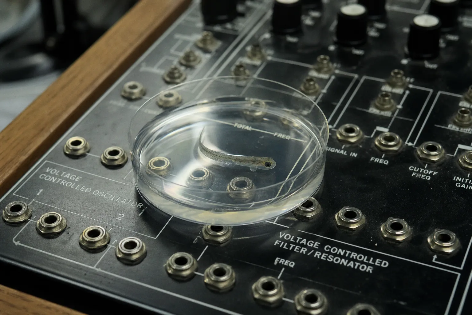
The difficult part is building a translation that remains intelligible when the data is noisy, the audience is moving through a gallery, and the installation has to run for hours without supervision.

For neuroaesthetics researchers working with zebrafish neurobiology, MIDI is a useful middle layer. It is small, widely supported, and familiar to the software already used in performance and installation work. A stream of notes can carry changes in timing, pitch, velocity, duration, and channel without requiring the neural recording itself to be treated as musical notation. This makes MIDI less a finished composition format than a practical event protocol between an analysis script and a sound engine.

The central question is therefore not whether neural activity can become sound. It can. The question is how much of the original signal to preserve, which features to make audible, and how quickly the translation needs to respond. The best neural data to MIDI conversion tools are not the ones that produce the most notes. They are the ones that make the chosen relationship between biological event and musical event clear enough to be heard.

Mapping Neural Events to Musical Protocols: Python Frameworks

Python remains the most direct route from a neural recording to a MIDI file or live MIDI stream. It is particularly useful in laboratory settings because preprocessing, analysis, mapping, and export can sit in the same environment. A researcher can work from spike times, local field potential envelopes, calcium-imaging traces, or already extracted event markers without moving immediately into a performance application.

Three tools are often considered for different parts of this workflow: music21, MIDITime, and midiutil. They are not interchangeable, and treating them as one stack can create unnecessary confusion.

music21 is a broad music-analysis and notation toolkit. It represents musical material as structured objects and includes its own MIDI import and export facilities. That distinction matters: music21 does not need to delegate MIDI file output to midiutil. For neural sonification, its strengths are the ability to organize notes and streams, manage durations and simultaneous events, and inspect or transform the musical result before export.

A typical mapping might begin by dividing a spike train into time windows. The number of events in each window becomes a firing-rate estimate; that value can then control pitch, velocity, or note density. An LFP envelope can be treated differently, perhaps as a slowly changing parameter for register or sustained amplitude. The data does not have to be forced into a melody. Several channels can be placed on separate MIDI channels or tracks, allowing bursts in different regions to form a chord-like texture.

The familiar MIDI pitch numbers provide a convenient reference. Pitch 60 is Middle C, while 21 corresponds to A0 on a standard 88-key piano. These values are not scientific categories; they are simply coordinates. The meaningful decision is the mapping around them: whether activity in the optic tectum should occupy a narrow central register, whether different brain regions should be separated by octave, and whether an event should create a new note or alter the parameters of one already sounding.

MIDITime is more specialized. It was designed for translating time-series data into MIDI and can be useful when the input is already represented as timestamped events. It suits quick experiments in which peaks, intervals, or other extracted features become notes. Its narrower scope can be an advantage when the goal is to test a mapping rapidly rather than build a complete musical-analysis layer.

midiutil is a lower-level MIDI file-writing library. It is appropriate when the researcher wants to construct tracks and events directly, with fewer abstractions between the data and the resulting file. It can be useful for simple exports or for a custom pipeline that needs explicit control over note messages and track structure. It should not, however, be described as the hidden output layer beneath every higher-level Python music library. The libraries differ in how they represent and write MIDI, and the choice should follow the required level of control.

A clean Python sonification pipeline treats MIDI not as a music format but as a structured event log. Pitch, velocity, duration, and channel are four axes onto which a multivariate neural signal can be projected.

A practical prototype might load spike-sorted data from an NWB file or a CSV export, divide events into windows, calculate a rate per channel, normalize the values to a chosen pitch range, and write a Type-1 MIDI file with separate tracks for selected electrodes or regions. The exact window size should follow the temporal question rather than a generic recipe. A short window preserves rapid bursts but can produce unstable note activity; a longer window produces a smoother line while hiding the timing relationships that may be the point of the sonification.

The same principle applies to normalization. Mapping every dataset independently to the full available range can make unrelated recordings sound deceptively similar. A fixed range based on a reference session may preserve comparability, while a session-specific range may be better for a single public demonstration. Either choice should be documented. A listener does not need to see the normalization equation, but the researcher needs to know what the resulting pitch or velocity actually represents.

Choosing the event model

There are several reasonable ways to represent neural activity in MIDI:

• One event, one note: useful for sparse spikes or clearly segmented responses, but potentially too busy for dense recordings.
• Windowed activity: converts a count or average into notes at regular intervals and produces a more stable texture.
• Continuous control: uses MIDI controllers, pitch bend, or an external parameter to represent a signal that should not be broken into discrete notes.
• Layered mapping: assigns different features to different musical dimensions, such as event timing to onset, firing rate to velocity, and region identity to channel.

The last option often gives the audience more to hold onto. A single signal mapped simultaneously to every musical parameter may appear expressive in a technical demonstration but become unreadable in a room. Separating roles makes it easier to hear what has changed when the biological input changes.

From Raw Audio to Polyphonic MIDI: Leveraging Spotify’s Basic-Pitch

Not every project begins with spike times. Some public-facing experiments first turn a neural signal into audio and then want to recover a manipulable musical representation. The source might be a filtered electrophysiology recording, the audio output of an earlier sonification stage, or a recording created by an interactive exhibit. In that situation, the problem runs in the opposite direction: sound is already present, and the researcher wants MIDI events that can be edited, routed, or reorchestrated.

Basic Pitch, developed by Spotify’s Audio Intelligence Lab, is designed for automatic music transcription. It uses a learned model to estimate note events from audio and can produce polyphonic MIDI, including overlapping notes and pitch-bend information where the transcription supports it. It is useful when the audio contains several simultaneous components and a simple monophonic pitch tracker would reduce the material to a single dominant line.

That does not make Basic Pitch a general neural-data interpreter. Its model was built for audio-to-note transcription, not for understanding action potentials, LFPs, or calcium signals as biological phenomena. The audio entering the system must already have enough pitch-like structure for transcription to be meaningful. A dense broadband signal may yield a technically valid MIDI file while still producing a poor representation of the underlying neural process.

The distinction is important in public work. If neural activity has been sonified as a set of pitched voices, Basic Pitch may help recover those voices. If the input is merely a raw or lightly filtered recording, the resulting notes should be treated as an exploratory transcription, not as a direct readout of neural events.

Basic Pitch can be used as a Python module or from the command line, depending on the surrounding workflow. It supports common audio formats, but format support is not the same as guaranteed transcription quality. Sample rate, noise, amplitude, filtering, and the amount of silence around an event all affect what the model can detect. A short, carefully prepared audio excerpt is usually easier to inspect than a long recording submitted without preprocessing.

The tool does not provide the kind of musical cleanup sometimes attributed to it. Basic Pitch does not, by itself, offer a built-in snap-to-scale and snap-to-beat workflow that should be credited for making an output musical. Its job is to infer note events from audio. Scale constraints, beat alignment, and stylistic regularization belong in a later stage: NeuralNote, a DAW, or a custom processing patch can perform those operations after transcription.

NeuralNote is relevant precisely because it places that later stage closer to the user. Distributed as a plugin and standalone application, it combines audio transcription with a piano-roll-oriented workflow in which detected notes can be inspected and adjusted. Depending on the version and host, quantization and other edits can be applied after the notes have been inferred. That makes it a practical bridge between an audio recording and a DAW session, especially when the exhibit team needs to revise the musical result without rewriting the entire analysis pipeline.

The editing step should remain visible in the research record. If notes are moved to a scale or snapped to a rhythmic grid, the final MIDI is no longer a neutral transcription of the input. That is not a flaw. It is an artistic and perceptual decision. The mistake is to present the cleaned version as though the neural signal itself arrived already organized into a key and meter.

Transcription and sonification are different acts. Basic Pitch can help recover note-like events from audio; it does not decide which biological feature deserves to become a note.

For an exhibition, the most convincing approach is often to keep two layers. One layer preserves the unquantized or minimally processed result, while another applies the musical constraints needed for the room. Visitors hear a stable and legible performance, while the research team can still compare it with the less edited source.

Real-Time Integration: Piping Neural Streams into Ableton Live

A MIDI file is useful for rehearsal, comparison, and a scheduled performance. A live installation needs something else: a stream that responds while the biological recording is being acquired. This changes the engineering problem. The pipeline must handle incomplete data, pauses, bursts, reconnects, and the ordinary unpredictability of a public space.

A common arrangement uses a Digital Audio Workstation as the performance host. Ableton Live is a popular choice because it can receive MIDI, route it to instruments, and host Max for Live devices for custom control. It is not the only possible host, but it provides a familiar environment for the final stage of an installation.

The architecture usually contains four functional layers:

1. Data acquisition. A recording system such as Open Ephys, an Intan-based setup, or a custom acquisition device produces spike events, band-limited signals, or extracted features. The connection may use USB, UDP, OSC, or another protocol supported by the hardware and software.

2. Parsing and mapping. A Python process, Pure Data patch, or dedicated application receives the data, applies the chosen windowing and normalization, and decides when to create, update, or release a musical event.

3. MIDI transport. The resulting messages are sent through a virtual MIDI port, an operating-system audio connection, or a device that bridges the data stream to the DAW.

4. Sound generation. Ableton or another host routes the messages to a synthesizer, sampler, granular instrument, or effect chain.

The important design decision is where to put state. A script that sends a note-on message for every detected event may work in a short test and fail in a gallery because notes accumulate, channels become saturated, or a momentary data dropout leaves a sustained sound hanging. A more robust system tracks active notes, imposes a maximum duration, and defines what happens when the incoming stream stops. Silence should be an intentional state, not an accident caused by a crashed process.

Max for Live can be used to build a custom receiver or to transform incoming MIDI inside Ableton. It should not be described as though a standard midi.quantize object automatically solves timing correction. Beat quantization can be implemented with a custom Max patch or with Ableton’s downstream MIDI and groove tools, but those are separate processing decisions. The incoming neural events still need to be timestamped and buffered appropriately before they can be aligned to a musical grid.

Other DAWs can perform the same role. Waveform Free and other hosts support MIDI routing and virtual instruments, although the exact device and plugin workflows differ. The choice is often determined less by absolute capability than by the team’s familiarity with the software, the licensing conditions of the venue, and the reliability of the available machine.

Latency should be measured as a chain, not guessed from the DAW alone. Acquisition, feature extraction, buffering, operating-system scheduling, virtual MIDI transport, instrument response, and audio output all contribute. A setup may feel immediate for a slow envelope mapping and noticeably delayed for a rapid spike-to-note mapping. The relevant test is perceptual: does a visible stimulus and its sonic consequence appear connected to an audience member, and does the connection remain stable after the installation has been running?

For many public events, a small buffer and a modest event rate are more valuable than an ambitious low-latency configuration. A system that occasionally drops a note or overloads the audio thread is less convincing than one that responds a little more slowly but remains predictable. Closed-loop experiments have stricter requirements and may call for dedicated acquisition or audio hardware. A gallery sonification should not borrow those requirements without also inheriting their engineering discipline.

Optimizing Data for Public Installations: Quantization and Scaling

A sonification that is useful to a researcher can be exhausting for everyone else. A recording may contain many channels, fine temporal structure, and large fluctuations that are meaningful in analysis but impossible to follow through loudspeakers. Public presentation is therefore a problem of controlled reduction.

Channel selection is usually the first decision. Several streams can be heard as a group, but only a limited number can be followed individually in a busy room. Choose channels because they support the explanation of the exhibit: one region may represent sensory input, another may respond to a visual stimulus, and a third may provide a contrasting background. If every available channel is included merely because it exists, the result is likely to sound dense without becoming more informative.

Pitch scaling is the next decision. MIDI provides 128 nominal pitch values, but a public installation rarely needs the whole range. A narrow register makes relationships easier to hear and prevents the output from jumping between extremes. A two-octave span can be effective, but the right range depends on the loudspeakers, the room, and whether the sound is meant to sit beneath speech or function as a central performance.

Scale restriction is also a downstream choice, not a property of the neural signal. A pentatonic or diatonic mapping can reduce accidental dissonance and make patterns easier to recognize. It can also hide differences if every value is forced into a small set of pitches. One useful compromise is to keep the event timing and velocity relatively faithful while restricting only the pitch set. Another is to maintain a continuous pitch mapping for one highlighted signal and use a constrained scale for supporting layers.

Quantization requires the same caution. Neural events are not normally organized around a bar line. Aligning them to a beat can make a piece easier to hear, but it changes the temporal representation. In a live workflow, quantization can be applied after event generation in Ableton’s MIDI tools, through a groove or timing process, in NeuralNote when working from transcribed audio, or in a custom patch. It should not be attributed to Basic Pitch or to a generic Max object that does not provide that function.

A useful installation may offer both timings at once: a direct layer that preserves the irregularity of the recording and a secondary musical layer that is lightly aligned to a pulse. The audience hears a coherent composition, while the tension between the two layers keeps the biological source from disappearing into a rigid beat.

Velocity curves are easy to overlook. A direct linear mapping from firing rate or amplitude to MIDI velocity often bunches most events into a narrow perceptual band. A logarithmic, square-root, or piecewise curve can make smaller changes audible without allowing occasional peaks to dominate the entire mix. The curve should be inspected against the distribution of the actual recording. A mathematically elegant transformation may still be wrong for a dataset with long quiet periods and rare bursts.

The same applies to silence. If low activity always produces a faint note, the installation never rests and the audience loses the significance of an event. A threshold, hysteresis, or minimum-duration rule can distinguish meaningful activity from background fluctuations. These rules should be chosen with care: too much gating produces an artificially sparse result, while too little makes every technical artifact part of the composition.

A compact mapping plan can be written as a set of explicit decisions:

• Which neural feature controls onset: a spike, a threshold crossing, a windowed count, or a smoothed envelope?
• Which feature controls pitch, and is the relationship linear, logarithmic, or scale-constrained?
• Does channel identity remain audible through MIDI channel, register, timbre, or spatial placement?
• What happens during missing data, an overloaded buffer, or a sudden amplitude spike?
• Which transformations are made for scientific fidelity, and which are made for audience comprehension?

Effective public sonification is a series of deliberate lossy compressions. Each cut — fewer channels, a narrower register, edited timing — trades completeness for perceptual clarity. The trade is usually worth making, but it should never be hidden.

Technical Constraints in Live Neuro-Art Exhibitions

The practical limits of a live installation are often less glamorous than the mapping itself. A patch can be conceptually elegant and still fail because of file size, clock behavior, audio routing, or the way visitors interact with the equipment.

Data ceilings appear when a tool expects short arrays or small event batches. A modest EEG excerpt may be easy to process, while a high-channel-count recording sampled at a high rate can exceed the assumptions of a teaching-oriented sonification tool. The answer is usually preprocessing: downsample a signal that does not need its original rate, extract events before transmission, or divide the recording into windows. The reduction should happen before the performance layer becomes responsible for carrying data it cannot use musically.

File-format compatibility is another quiet source of failure. Audio transcription tools and DAWs may accept many formats in principle, while a particular plugin, driver, or older patch accepts only a subset. A standardized internal format makes troubleshooting easier. For audio, an uncompressed WAV exchange file is often simpler than repeatedly converting between compressed formats. For neural recordings, the installation should receive a documented feature stream when possible rather than a full raw acquisition file that the performance computer must interpret in real time.

Clock drift matters in any exhibit that aligns sound with video, microscopy, animation, or a visitor-controlled stimulus. The acquisition system and the DAW may each maintain their own clock. Over a long session, small differences can accumulate into a visible or audible misalignment. A periodic synchronization message, shared timestamp, or heartbeat can help the software detect and correct that divergence. If exact alignment is not necessary, the artwork may instead be designed so that the sound remains meaningful without pretending to be frame-accurate.

Recovery behavior deserves to be tested in public conditions. What happens when the USB device disconnects? Does the DAW continue producing a safe background texture, or does it stop with an error? Can the operator restart the parser without restarting the audio host? Does the system save the last valid state, and can it distinguish a genuine period of low neural activity from a broken connection? These are not merely IT questions. They determine whether the audience experiences an intentional pause or a technical failure.

Audio levels and room acoustics can distort the mapping as much as the code does. A narrow frequency range may disappear under ventilation noise, while sharp transients can become unpleasant near a wall or in a reflective gallery. A loudness envelope that works on headphones may overwhelm a room. The installation should be calibrated in the space where it will be heard, with the visual content and expected audience distance included in the test.

Audience bandwidth is the constraint that rarely appears in a methods section. Visitors do not listen to a neural sonification the way they inspect a plot. They enter at different times, may stay for only a minute, and may be talking while the sound changes. The installation therefore needs a perceptual entry point: one channel that follows a visible event, one recurring timbre, or one transition that makes the mapping legible. Other neural streams can provide texture, but they should not compete with the one relationship the audience is meant to understand.

The zebrafish offers a particularly useful case because its nervous system can be presented through several simultaneous representations: microscopy, movement, neural activity, and sound. The danger is allowing the music to imply more certainty than the measurement supports. A low note should not be presented as though the animal is literally producing that pitch in its brain. It is a chosen encoding of a measured feature. Clear labels and a visible mapping explanation protect the work from becoming a misleading spectacle without forcing the installation to turn into a lecture.

From Spike Train to Standing Ovation

The route from a recording electrode or imaging trace to a gallery loudspeaker is technically accessible, but accessibility does not remove the need for judgment. Python can handle the analytical translation; music21 can organize and export MIDI through its own I/O; MIDITime or midiutil may suit narrower or lower-level workflows; Basic Pitch and NeuralNote can support an audio-to-MIDI round trip when the source is already sound-like; and Ableton Live or another DAW can provide the performance layer.

The important work is deciding what each stage is allowed to change. A spike train can become a sequence of events, but it does not arrive with a natural key. An LFP envelope can control a filter or a sustained tone, but it does not automatically imply a melody. An audio transcription model can infer overlapping notes, but it does not tell the researcher whether those notes remain a faithful representation of the original neural process. Quantization can make an installation easier to hear, while also moving events away from their recorded timing.

For a public prototype, the most reliable starting point is deliberately small: one recording, one selected feature, one mapping, and one clear auditory consequence. Compare the raw and processed versions. Test the system with missing data. Listen in the exhibition space rather than only in headphones. Then add channels or musical constraints one at a time, keeping track of which change improves comprehension and which merely adds activity.

A successful installation does not make the neural data sound conventionally musical at every moment. It gives the audience a stable way to notice change. Sometimes that means preserving irregularity; sometimes it means placing a soft grid beneath it. Sometimes the most honest result is a sparse sequence with long silences. The point is not to disguise biology as composition, but to construct a form in which biological variation can be perceived.

The zebrafish will continue to move whether anyone is listening. Public neuroaesthetics begins when the translation makes that activity available to the ear without pretending that an artistic encoding is the same thing as the measurement. The strongest neural data to MIDI conversion tools are therefore not those that automate interpretation. They are the ones that leave the researcher enough control to make the choices visible, testable, and worth hearing.