Habenular circuit mapping: a 4-step optogenetic protocol
Habenular circuit mapping fails at the first bottleneck more often than at the microscope. If opsin expression is not restricted to the intended habenular subregion, every downstream result becomes difficult to interpret.
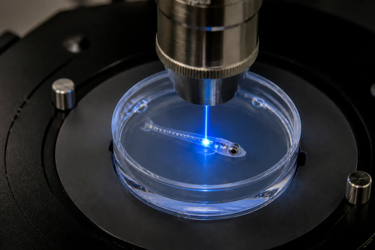
A clean behavioral phenotype cannot rescue a contaminated projection map.
The workable sequence is strict: define the source population, deliver and validate the opsin, stimulate the projection with calibrated timing, then align physiological readouts with behavior. In zebrafish, the implementation may use transgenic driver lines, Gal4/UAS or Cre/lox systems, targeted transgenesis, and larval optical access rather than the viral strategies common in mammalian preparations. The logic does not change. Isolate. Stimulate. Record. Quantify.
The protocol is only as good as its spatial restriction. Light gives temporal precision; genetic targeting supplies the circuit identity.
Step 1: Define the habenular source population before delivering the opsin
The habenula is not a single functional node. The medial and lateral divisions differ in projection targets, neurotransmitter content, developmental organization, and behavioral output. A protocol that labels the entire habenula may produce a strong signal and still answer the wrong question.
Start by fixing the circuit boundary.
For a habenulo-interpeduncular pathway activation experiment, the source population is the habenular subdivision and the target is the interpeduncular nucleus, or IPN. For avoidance-related experiments, the projection may instead be mapped toward midbrain targets such as the rostromedial tegmental nucleus in mammalian systems. In zebrafish, anatomical homology and nomenclature require care. Do not transfer a mammalian target map into a larval fish without confirming the corresponding structure and projection geometry.
The first design pass should specify:
- Source region: medial habenula, lateral habenula, or a defined neuronal subpopulation.
- Target region: IPN, midbrain, or another anatomically identified downstream area.
- Direction of manipulation: activation of cell bodies, axons, or presynaptic terminals.
- Readout: evoked current, calcium response, synaptic marker, locomotor output, avoidance, or social behavior.
- Developmental stage: larval, juvenile, or adult preparation.
- Circuit state: intact animal, acute brain preparation, spinal preparation, or slice.
This sounds administrative. It is not. The same opsin can answer different questions depending on where the light is delivered. Stimulating habenular somata tests the effect of recruiting the source population. Stimulating terminals tests the contribution of a defined projection. Stimulating fibers of passage can create a third experiment without announcing it.
Choose expression logic that matches the question
A Cre-dependent viral vector such as AAV-FLEX-ChR2 can restrict expression to Cre-positive neurons in a selected region. That approach is common in mammalian circuit work. Zebrafish experiments more often rely on stable driver lines, Gal4/UAS systems, enhancer traps, or cell-type-specific promoters. Each system introduces its own leakage profile.
The operational rule is simple: expression logic must be validated in the exact line, age, and tissue preparation used for the experiment.
A promoter that appears selective in a published atlas may broaden during development. A driver line may label a neighboring habenular population at one stage and become more restricted later. A viral injection may spread along a ventricle or white-matter tract. The map must show what was actually labeled, not what the construct was designed to label.
For each animal or preparation, quantify at least:
1. The fraction of opsin-positive cells located inside the intended habenular subregion.
2. The fraction of labeled cells outside that region.
3. The projection pattern at the downstream target.
4. The overlap between opsin expression and the neuronal marker used to define the population.
5. The number and distribution of labeled axons near the stimulation site.
The last point matters for terminal stimulation. Dense fluorescence in the source region does not prove that the target contains functional labeled terminals. Conversely, sparse terminal labeling can still produce measurable synaptic responses if the projection is strong and the stimulation is well calibrated.
Build the anatomical map before functional testing
Use a structural marker or reporter to establish the path from habenula to target. In a zebrafish preparation, confocal imaging can provide the initial projection map. Two-photon imaging becomes useful when the experiment requires deeper optical access, longitudinal tracking, or simultaneous activity measurements.
Do not use a positive fluorescence image as a substitute for projection specificity. A labeled axon in the target region indicates transport and anatomy. It does not prove synaptic release. Functional connectivity requires a physiological response that follows the optical stimulus with appropriate timing and depends on the intended pathway.
The anatomy also determines the stimulation geometry. If habenular terminals occupy a compact subregion of the IPN, place the stimulation field there. If the projection branches broadly, define a reproducible region of interest and report it. The light path, focal depth, and illuminated volume are part of the experiment, not incidental microscope settings.
Step 2: Calibrate optical stimulation at the presynaptic projection
Channelrhodopsin-2 is commonly activated with blue light around 473 nm. Its practical value in circuit mapping comes from temporal control: millisecond-scale pulses can recruit presynaptic terminals and align the resulting response with electrophysiological or calcium signals.
The wavelength is only one parameter. The actual stimulus depends on:
- pulse duration;
- pulse frequency;
- train length;
- inter-trial interval;
- illuminated area;
- focal depth;
- objective transmission;
- tissue scattering;
- opsin expression level;
- temperature and preparation state.
There is no universal light power density that can be transferred between rigs without calibration. Optical output at the objective is not equivalent to irradiance at the target tissue. A larval zebrafish brain, an acute slice, and an adult in vivo preparation will attenuate and distribute light differently.
Measure the optical output at the plane that matters. If the experiment uses a focused beam, characterize the focal spot and axial spread. If it uses wide-field illumination, define the illuminated region and account for neighboring structures. Record the settings with enough precision that another operator can reproduce the stimulus without reconstructing the setup from memory.
Separate cell-body stimulation from terminal stimulation
The most direct test of a projection is terminal stimulation in the downstream target. Delivering light to habenular axons in the IPN, for example, reduces the chance that the response originates from unrelated collaterals activated at the source. It does not remove every confound. Axons may branch. Light may reach nearby fibers. Opsin expression may be ectopic.
Cell-body stimulation remains useful when the goal is to assess population-level recruitment or behavioral causality. But it is less specific as a synaptic connectivity assay. State the distinction in the protocol and keep the two manipulations analytically separate.
A basic stimulation matrix can be organized as follows:
| Parameter | Terminal mapping | Cell-body recruitment |
|---|---|---|
| Light location | Downstream target, such as IPN | Habenular source region |
| Primary question | Does the projection drive a postsynaptic response? | What is the effect of recruiting the source population? |
| Main risk | Activating nearby axons or collaterals | Recruiting multiple projections from the same neurons |
| Best paired readout | Patch-clamp current or local calcium response | Calcium activity, locomotion, avoidance, or social behavior |
| Interpretation | Projection-level function | Population-level function |
Use short pulses first. A single pulse can reveal latency, response polarity, and trial-to-trial reliability. Longer trains can test temporal integration but also increase the chance of depolarization block, synaptic depression, heating, and behavioral adaptation.
For presynaptic activation, verify that the response follows the expected time course and survives repeated trials within a defined stability window. If the response declines rapidly, do not automatically interpret that decline as circuit adaptation. It may reflect synaptic depression, photobleaching, tissue drift, declining cellular health, or a change in optical alignment.
Control the geometry, not only the genotype
A no-opsin control exposed to the same light pattern tests light-related effects. A no-Cre or no-Gal4 control tests expression that depends on unintended recombination or driver activity. These controls address different failure modes.
Use the same objective, wavelength, pulse structure, and stimulation location in control preparations. If the control receives a weaker or differently focused stimulus, it does not isolate the optical artifact.
Leaky transgene expression deserves separate attention. Chrimson and related actuators can generate off-target fluorescence or stimulation effects when expression escapes the intended genetic gate. In calcium imaging, the actuator can also interfere with the indicator signal through spectral overlap, direct excitation, or local photophysical artifacts. A visually clean trace is not evidence that the signal is clean.
Step 3: Combine electrophysiology with calcium imaging
Optogenetic circuit mapping is strongest when two readout layers converge. Electrophysiology provides temporal precision and synaptic kinetics. Calcium imaging provides spatial coverage and cell-population structure. Neither should be treated as a complete map on its own.
Use patch-clamp recordings to establish synaptic connectivity
To test a monosynaptic connection, record from neurons in the downstream target while stimulating labeled habenular terminals. In the IPN, for example, a light-evoked postsynaptic current that appears with short and consistent latency is compatible with direct projection input. The response must still be tested against network-mediated explanations.
A practical sequence is:
1. Establish a stable recording from a target neuron.
2. Deliver a single optical pulse to the labeled projection.
3. Measure response latency, amplitude, polarity, and trial reliability.
4. Repeat at different holding potentials where the preparation permits.
5. Apply synaptic transmission blockers or pathway-specific controls where appropriate.
6. Compare responses in opsin-positive and negative-control preparations.
7. Map multiple target neurons rather than selecting only visibly responsive cells.
The output is not simply responsive versus nonresponsive. Quantify the distribution of response amplitudes, the proportion of connected target cells, latency variability, failure rate, and spatial location within the target nucleus.
If a postsynaptic current is detected, distinguish excitatory and inhibitory components. Habenular projections can engage different transmitter systems, and cholinergic and glutamatergic signaling may coexist in the same pathway. A response that looks excitatory at one holding potential may include mixed components or polysynaptic recruitment.
The cleanest map reports the pharmacological and voltage-clamp logic used to separate those components. Avoid collapsing a mixed response into a single label such as excitatory pathway. The circuit may release more than one transmitter, or recruit local interneurons that reshape the recorded current.
Add calcium imaging for spatial distribution
GCaMP imaging can reveal which neurons across the target region respond during optical stimulation. This is valuable when the target contains intermingled cell types or when patching would sample too few cells.
Align the imaging frames to the optical pulse with millisecond-accurate timestamps. Define the baseline window before stimulation, the response window after stimulation, and the exclusion criteria for motion or unstable fluorescence. Use the same preprocessing pipeline across experimental and control groups.
Quantify:
- response probability per cell;
- peak ΔF/F;
- response latency;
- rise and decay time;
- spatial clustering;
- trial-to-trial consistency;
- relationship between calcium response and anatomical cell class.
Calcium signals integrate activity over time. They do not provide the same temporal resolution as patch-clamp recordings. A delayed GCaMP response does not necessarily indicate delayed synaptic transmission. It may reflect indicator kinetics, intracellular calcium handling, or network recruitment.
Calcium imaging expands the map. It does not replace the timing information needed to prove direct connectivity.
Treat optical artifacts as a primary variable
Optical stimulation and calcium imaging share the same physical environment. Blue light used for ChR2 activation can contaminate fluorescence measurements. Red-shifted actuators may reduce some spectral conflicts but introduce their own risks, including leaky expression and actuator-dependent artifacts.
The control framework should include, where feasible:
- indicator-positive, opsin-negative tissue exposed to the stimulation light;
- opsin-positive, indicator-negative tissue to characterize direct optical effects;
- no-Cre or no-Gal4 animals;
- no-light trials;
- stimulation at a nearby non-projecting region;
- trials with altered pulse timing but matched light exposure.
Inspect raw fluorescence traces. Do not rely only on processed ΔF/F plots. A stimulus-locked jump that appears in every region of interest, including cells outside the anatomical projection, is likely an optical or motion artifact. A response that scales with projection density and disappears in genetic controls is more consistent with pathway-dependent activity.
For quantitative mapping, establish an artifact threshold before analyzing the experimental group. The threshold should be based on the control distribution, not chosen after inspecting the strongest responding cells.
Step 4: Connect circuit activation to behavior without overextending the map
A physiological connection is not automatically a behavioral mechanism. Slice data can identify synaptic input. Whole-animal stimulation can test whether that input contributes to an action or state. The two experiments answer different questions.
Activation of lateral habenular projections to midbrain structures has been associated with active, passive, and conditioned avoidance in behavioral paradigms. The specific outcome depends on the stimulated projection, pulse pattern, developmental stage, baseline state, and behavioral assay. Do not treat all avoidance-like behavior as evidence for one conserved circuit operation.
Select the behavioral assay to match the circuit claim
For zebrafish, candidate readouts may include locomotor suppression, escape-like movement, place preference or avoidance, social interaction, habituation, and stimulus-contingent choice. Select one primary endpoint before collecting data.
A useful behavioral protocol defines:
- the baseline observation period;
- the stimulation period;
- the post-stimulation period;
- the optical stimulus pattern;
- the arena geometry;
- the tracked variables;
- the exclusion rules;
- the blinding or automated scoring method.
Quantify behavior as a time series rather than a single endpoint whenever possible. Track velocity, distance moved, turning rate, freezing duration, occupancy, inter-animal distance, or zone transitions according to the assay. A reduction in total distance can reflect freezing, motor impairment, sedation, visual disruption, or generalized circuit inhibition. The same number can support different biological interpretations.
Use sham stimulation and opsin-negative controls. If the experiment claims projection specificity, compare terminal stimulation with source-region stimulation. If the experiment claims transmitter-specific function, pair the behavioral test with a physiological validation of the manipulated synapse.
Keep developmental biology in the design
The habenulo-interpeduncular pathway changes across development. Axon guidance, neuronal migration, synaptic maturation, and transmitter expression do not proceed as independent modules. A projection can be anatomically present before it is functionally mature. A behavioral output can change while the gross projection remains stable.
For a zebrafish neural circuit study, report the developmental stage with precision and use stage-matched controls. Larval transparency improves optical access but does not guarantee mature circuit function. A response observed early in development may reflect a transient network configuration rather than the adult pathway.
This is also where a habenular axon guidance assay can complement optogenetic mapping. If the experimental question concerns circuit assembly, first quantify path selection, terminal distribution, or midline crossing. Then test functional transmission. A malformed projection and a silent synapse are not interchangeable phenotypes.
Distinguish correlation from causal recruitment
A calcium response during a behavioral event shows co-activation. Optogenetic stimulation can test causal influence, but only if the stimulation is restricted and the behavioral analysis is calibrated.
The causal chain should be explicit:
1. Opsin expression identifies the source population or projection.
2. Light recruits that population with a defined temporal pattern.
3. Electrophysiology or calcium imaging confirms downstream engagement.
4. Behavior changes during or after the stimulation.
5. Controls exclude light, driver, expression, motion, and general arousal effects.
If step three is missing, the behavior may result from unintended recruitment. If step four is missing, the circuit map remains physiological rather than behavioral. If step five is missing, the phenotype cannot be assigned confidently to the habenular pathway.
What the final dataset should contain
A robust experiment produces aligned anatomical, physiological, optical, and behavioral records. Avoid building the result around one representative image or one responsive neuron.
At minimum, organize the dataset around four linked objects:
- Expression map: source cells, off-target labeling, terminal density, and developmental stage.
- Optical calibration record: wavelength, pulse timing, illumination geometry, measured output, and stimulation location.
- Connectivity map: target cells sampled, response probability, latency, amplitude, transmitter components, and controls.
- Behavioral record: baseline, stimulation, post-stimulation measurements, individual trajectories, and exclusion decisions.
The analysis should preserve animal-level structure. Cells are nested within preparations. Trials are nested within animals. Treating every cell or every trial as an independent biological replicate inflates apparent sample size and can produce an unstable result. The unit of inference must match the experimental design.
For circuit mapping, report both positive and negative evidence. A target region with no evoked response is informative only if expression, illumination, recording quality, and synaptic viability were verified. A weak response is not necessarily a failed experiment. It may indicate sparse connectivity, restricted release probability, poor terminal access, or a subpopulation mismatch.
A strict troubleshooting sequence
When the map is inconsistent, do not modify several parameters at once. Isolate the failure in the order that the signal is generated.
1. Confirm expression
Inspect the source region and the downstream projection. Check for leakage beyond the intended habenular subdivision. Verify the driver genotype and reporter pattern. If the expression map is wrong, stop there.
2. Confirm light delivery
Measure the optical output and inspect the focal plane. Recheck the target location after the experiment. A small shift can move stimulation away from terminals or onto adjacent fibers.
3. Confirm actuator function
Use a direct response assay appropriate to the preparation. A failed response may reflect inactive opsin, poor membrane trafficking, insufficient expression, or tissue damage. Do not interpret a silent circuit until actuator performance is established.
4. Confirm recording stability
Track baseline noise, access resistance, fluorescence drift, motion, and trial stability. Reject traces using criteria fixed before group comparison.
5. Confirm synaptic dependence
Test whether the response depends on the expected synaptic pathway. Compare latency and waveform across controls. Separate direct postsynaptic currents from network-mediated activity.
6. Confirm behavioral specificity
Run the same stimulation in opsin-negative and driver-negative controls. Compare locomotor capacity, visual function, and baseline arousal. A behavior that disappears when the projection is stimulated at a different location is more informative than a behavior that simply follows any intense illumination.
The sequence prevents a common analytical mistake: troubleshooting the behavior when the actual defect is anatomical or optical.
Final protocol parameters
A practical habenular circuit mapping optogenetic protocol should close with a compact parameter record, not a broad claim of reproducibility.
Record:
- the source subdivision and target structure;
- the genetic or viral expression strategy;
- the opsin and indicator used;
- the developmental stage;
- the stimulation wavelength, commonly 473 nm for ChR2;
- pulse duration, frequency, and train structure;
- measured optical output at the tissue plane;
- stimulation location and illuminated volume;
- electrophysiological or calcium-imaging acquisition settings;
- behavioral assay and tracking variables;
- no-opsin, no-Cre or no-Gal4, and no-light controls;
- criteria for excluding unstable recordings or contaminated imaging traces.
The strongest circuit maps do not rely on a single technology. They triangulate. Anatomy establishes the route. Optical stimulation recruits it. Electrophysiology measures synaptic timing. Calcium imaging expands spatial coverage. Behavior tests functional consequence. Controls determine whether the signal belongs to the pathway or to the apparatus.
That is the practical standard: define the circuit narrowly, calibrate the light at the tissue, quantify every response layer, and refuse to call a projection functional until the controls survive the same stimulation.