Zebrafish Optogenetic Mapping: A Step-by-Step Lab Protocol
You can record calcium activity across the entire larval brain. That part is solved. The harder problem is assigning function to specific connections when your stimulator lights up hundreds of neurons at once and your sensor picks up the aggregate blur.
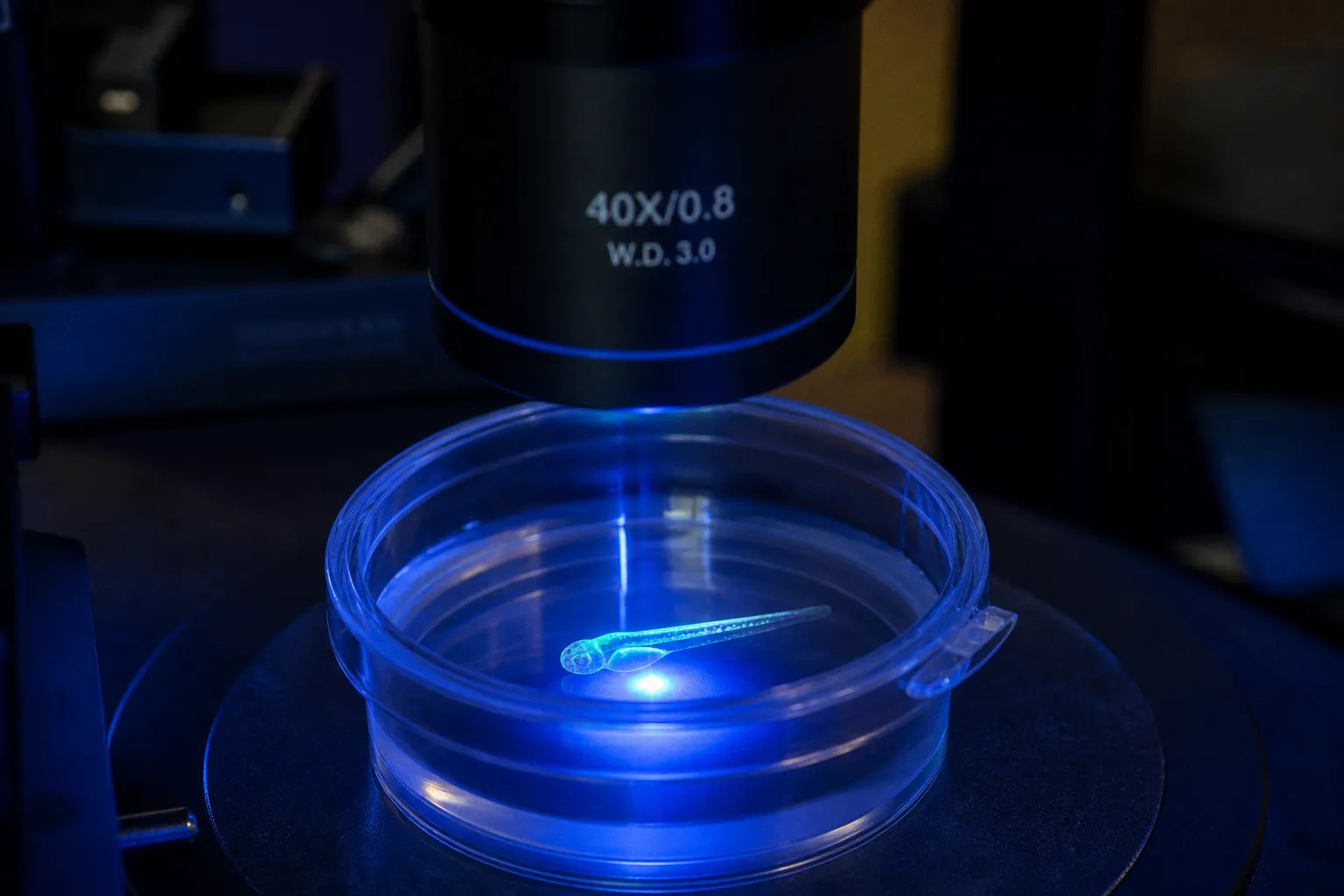
Sparse targeting resolves this — but only if you calibrate every step from stochastic labeling to spectral separation with mechanical precision. Miss one parameter and you are back to averaging noise.
This protocol is for the lab that wants to map functional connectivity in zebrafish with single-cell resolution. It brings together four workflows that are often treated separately: the Optobow system for sparse all-optical connectivity mapping, PA-Rac1-mediated axon guidance in embryonic motor circuits, optogenetic interrogation of the habenulo-interpeduncular pathway, and single-neuron photo-activation with phototoxicity control. The methods share the same basic demand: stimulation must be selective enough to identify a circuit, and the recording must be clean enough to show what that circuit actually did.
The practical details matter more than the headline technology. Expression patterns vary from larva to larva. A nominal wavelength does not guarantee spectral isolation. A clean-looking calcium trace can still be a motion artifact, a light artifact, or the consequence of an actuator that was already partially activated during preparation. The protocol works when those possibilities are treated as experimental variables rather than after-the-fact explanations.
The Optobow System for Sparse Functional Connectivity Mapping
The Optobow toolbox addresses a specific engineering problem: how to stimulate and record from nonoverlapping, sparsely labeled neuronal subsets within the same larva at the same time. It combines the Gal4-UAS transcription system with Cre/lox stochastic recombination to express the red-shifted optogenetic actuator ChrimsonR and the green calcium indicator GCaMP6f in disjoint neuronal populations. The result is a preparation in which one sparse group can be activated while another, broader population is monitored across the brain during the same imaging session.
That separation is what turns whole-brain imaging into circuit mapping. Without it, a stimulus can produce a large fluorescence response without revealing which cells were directly recruited, which cells were downstream, and which cells simply moved or changed state in parallel.
How the Labeling Works
The Gal4 driver line provides broad expression. Cre/lox recombination then stochastically removes one reporter and activates the other in individual cells. Because recombination is probabilistic, each larva carries a different sparse pattern. The useful preparation is therefore not defined by genotype alone. It is defined by the expression pattern that is actually present in the individual animal.
Screen for larvae in which the ChrimsonR-positive cells are sufficiently isolated and limited in number — typically fewer than twenty actuator-positive neurons — while the GCaMP6f population remains broad enough to provide a functional readout. The point is not to maximize labeling. It is to make the stimulated population interpretable. If too many ChrimsonR-positive cells sit close together, the experiment begins to resemble broadfield stimulation, even if the genetic design is technically sparse.
The screening step should also include the position of the labeled cells. A sparse pattern distributed across several unrelated regions may be less useful than a smaller group concentrated in the circuit under study. Record the anatomical identity and relative location of the actuator-positive neurons before stimulation. That information becomes important during analysis, especially when the optical spot or stimulation volume is larger than the soma of a single target.
Stochastic expression creates a necessary trade-off. Transient expression is mosaic and variable, and fluorescence intensity is not a reliable proxy for identical actuator abundance across animals. You cannot assume that two larvae with the same number of visible ChrimsonR-positive neurons will respond with the same optical gain. For each larva, verify both the expression pattern and the imaging quality before committing to a full connectivity run. This costs time at the front end and prevents the more expensive false negative: stimulating cells that barely express the actuator and concluding that the connection is absent.
Timing and Incubation
Standard incubation runs at 28.5 °C. Optobow connectivity mapping is typically performed at 5 days post-fertilization, when circuits have matured sufficiently for measurable synaptic transmission while the brain remains small enough for whole-brain light-sheet coverage. Earlier timepoints risk incomplete circuit formation. Later stages increase scattering and reduce imaging depth, making it harder to preserve a consistent signal across the field.
Temperature is not a background setting here. It affects development, movement, baseline physiology, and the timing of the response you are trying to measure. Confirm it with a calibrated probe rather than relying only on the incubator display. A small mismatch between the nominal temperature and the temperature at the preparation can become a systematic difference between batches.
Imaging Configuration
The spectral separation that makes all-optical interrogation possible depends on a simple constraint: ChrimsonR and GCaMP6f must not cross-talk. ChrimsonR has a red-shifted activation range centered around 590 nm, while GCaMP6f is commonly excited around 488 nm and emits in the green range. A light-sheet microscope with independent stimulation and imaging arms can handle the separation, but the instrument must be tested rather than trusted by design.
Run a negative control in a larva expressing GCaMP6f without ChrimsonR. Deliver the same stimulation pattern used in the experiment and monitor the green channel. Any time-locked fluorescence change indicates optical contamination, a stimulation-induced motion artifact, or another non-biological response. The control does not tell you which of those problems is present, but it tells you that the experimental trace cannot yet be interpreted as circuit activity.
The reciprocal control is equally important: stimulate ChrimsonR in the absence of GCaMP6f and image through the same optical path. This reveals whether stimulation light is being detected directly by the camera or leaking through the emission filters. Run both controls when the stimulation arm, filters, dichroic, laser alignment, or acquisition settings change.
The system only works if your stimulation and detection channels are spectrally airtight. One filter mismatch and you are measuring your own light, not the circuit's response.
In practice, the Optobow preparation is a balance between sparsity and signal. Too little actuator expression produces an apparently silent circuit. Too much expression increases the chance of recruiting neighboring cells and obscures the distinction between direct and indirect responses. Too narrow a recording field loses downstream activity. Too broad a stimulation field turns the experiment back into population activation. The useful range has to be established per preparation, not assumed from the construct name.
Precision Axon Guidance Using PA-Rac1 and Embryonic Mounting
Photoactivatable Rac1, or PA-Rac1, lets you steer axon growth with light. In embryonic zebrafish, this translates to real-time control over motor-neuron pathfinding: illuminate a defined region of the growth cone and bias the direction in which the axon extends. The method is powerful because it manipulates the geometry of development rather than merely recording the endpoint. You can ask not only whether a neuron reached its target, but how a local change in Rac1 activity altered the route.
The technique is particularly useful for caudal primary, or CaP, spinal motor neurons. Their axons extend into the periphery in a well-characterized sequence, providing a relatively clear system in which to compare stimulated and unstimulated growth trajectories.
Developmental Window
The practical stimulation window is 23–25 hours post-fertilization. This overlaps with the onset of heart beating at approximately 24 hpf, which provides a convenient developmental landmark during preparation. Before 23 hpf, CaP axons have not extended far enough for many pathfinding manipulations to be informative. After 25 hpf, major trajectory decisions are increasingly committed and the tissue becomes less responsive to local photo-activation.
The window should be treated as a biological condition, not merely a timestamp. Embryos at the same nominal age can differ in developmental progress depending on temperature and handling. Note the morphology of the embryo and the position of the growth cone when beginning stimulation. The later analysis depends on knowing whether a trajectory change occurred during active pathfinding or after the relevant decision had already been made.
Mounting Protocol
Mounting must immobilize the embryo without triggering PA-Rac1 activation before the experiment begins. Use 1% low-melting-point agarose dissolved in E3 medium containing 0.0168% tricaine anesthetic. Tricaine prevents tail movement during imaging. The agarose provides mechanical stability while remaining soft enough to avoid compressing the embryo or distorting the anatomy used to identify the motor neuron.
A useful mounting preparation keeps the target growth cone accessible to the stimulation path while leaving enough of the embryo visible to monitor general condition. Excess agarose can make optical access difficult. Insufficient agarose allows small movements that are easy to mistake for changes in axon trajectory. The correct mount is not the tightest one; it is the one that holds the embryo without adding pressure or obscuring the region being manipulated.
| Parameter | Value | Purpose |
|---|---|---|
| Agarose concentration | 1% LMP in E3 | Mechanical stability without compression |
| Anesthetic | 0.0168% tricaine | Prevents movement artifacts |
| Developmental stage | 23–25 hpf | CaP axons actively pathfinding |
| Incubation temperature | 28.5 °C | Standard zebrafish development rate |
Light Control During Setup
PA-Rac1 activates in the 400–500 nm spectrum. Standard room lighting can therefore trigger it before the intended stimulation sequence. All mounting and imaging setup must occur in a dark room using only light above 500 nm wavelength. Amber or red safe lights are suitable, provided the setup has been checked rather than assumed to be safe.
The imaging laser power should remain below 2% during non-stimulation periods. Exceeding that level can activate PA-Rac1 before the experimental baseline has been established. Once baseline activation has occurred, later illumination is difficult to interpret: a stimulated embryo may show little additional effect because the relevant signaling pathway has already been partially engaged.
This is a common protocol failure because the preparation itself looks harmless. The embryo is being mounted, not exposed to an obvious stimulation pulse, yet fluorescent room lights can deliver enough short-wavelength light to compromise the comparison. Keep the white lights off after PA-Rac1 embryos are mounted, use the approved safe light throughout setup, and verify with a spectrometer that the imaging system does not leak below 500 nm during alignment or low-power acquisition.
The control condition must be handled under the same light restrictions as the stimulated condition. Otherwise, the control is not testing the effect of photo-activation; it is testing a different preparation history.
Asymmetric Signaling in the Habenulo-Interpeduncular Pathway
The habenulo-interpeduncular, or Hb-IPN, pathway is a bilateral circuit with pronounced left-right functional asymmetry. That makes it a useful test case for optogenetic dissection. You can target one side and compare its behavioral contribution with the other side, but the pathway should not be reduced to a simple left-versus-right switch. The neurotransmitter composition and the timescale of the responses both matter.
Dual Neurotransmitter Signature
Stimulating channelrhodopsin-2 in the dorsal habenula generates two distinct postsynaptic currents in the ventral interpeduncular nucleus. The first is a fast glutamatergic excitatory postsynaptic current. The second is a slow-rising cholinergic current. Both arrive at the same target nucleus, but they occupy different temporal domains and may support different downstream computations.
This distinction should shape the recording protocol. If the recording window is too short, or if high-pass filtering removes slow components, the glutamatergic response will be visible while the cholinergic response disappears from the analysis. Use a recording window of at least 500 ms after the stimulus and choose filtering that preserves slow currents. A trace that returns to baseline quickly is not necessarily evidence that no slower signal occurred; it may simply reflect the way the acquisition was configured.
The two components can also complicate comparisons between animals. A preparation with a strong fast response and a weak slow response may have a different functional balance from one with the opposite profile, even if the peak amplitude looks similar. Record enough of the response to examine latency, rise time, duration, and recovery rather than reducing the pathway to a single maximum.
Behavioral Readout: Freezing and Resumption
The left dHb-IPN projection specifically modulates defensive behavior. Optogenetic activation of the left dHb in larval zebrafish reduces freezing duration and promotes rapid resumption of swimming following an electric shock. Conversely, severing the left dHb-IPN projection prolongs freezing.
This provides a clear behavioral assay, but the timing of the stimulus must be consistent. Stimulate the left dHb during or immediately after the shock pulse, then measure the time to resume swimming. Compare stimulated animals with unstimulated controls and with larvae in which the left projection has been physically severed. The difference between stimulated and severed conditions helps separate the pathway's contribution from general changes in arousal or motor capacity.
The behavioral readout should be paired with an anatomical and physiological check. A larva that fails to resume swimming may have an altered circuit response, but it may also be poorly positioned, partially immobilized, or affected by the mounting condition. The same preparation logic applies to the stimulation itself: confirm that the light is reaching the intended dHb population and not an adjacent structure.
The bilateral organization is useful only when the side of stimulation is treated as an experimental variable. Pooling left and right dHb stimulation too early can erase the asymmetry that makes the pathway informative. Keep the side, target coordinates, stimulation timing, and behavioral state associated with each trial during acquisition and analysis.
What This Pathway Is Not
The Hb-IPN pathway contains both glutamatergic and cholinergic projections. It is not purely cholinergic, despite the common simplification in review literature. A protocol that blocks only nicotinic receptors and declares the pathway silenced will leave the glutamatergic component intact. If the goal is to assign a behavioral effect to a specific signaling mode, use dual pharmacological blockade or confirm the result with optogenetic isolation of the relevant transmitter population.
The Hb-IPN pathway runs two neurotransmitter channels in parallel. Block one and you still have a live circuit — just a noisier, harder-to-interpret one.
This is also why pharmacology should not replace optical and anatomical controls. A residual response after receptor blockade may be a genuine second transmitter component, but it can also reflect incomplete drug access or an off-target effect. The interpretation becomes stronger when the timing of the residual signal matches the expected component and when the projection has been independently verified.
Mitigating Spectral Cross-Talk in All-Optical Whole-Brain Imaging
All-optical interrogation — simultaneous photo-stimulation and calcium imaging — demands that actuator and sensor occupy sufficiently separate spectral windows. The ChrimsonR/GCaMP6f pairing was designed for that purpose. ChrimsonR responds to red-shifted light around 590 nm. GCaMP6f is commonly excited around 488 nm and emits in the green range, around 510 nm. In principle, red stimulation and blue excitation remain distinct.
In practice, cross-talk enters through several routes. Some are optical. Others look optical but are actually photobleaching, heating, or motion. Treating all of them as the same problem makes troubleshooting slower.
Route 1: Stimulator Emission Bleed-Through
Red LEDs and lasers are not perfectly monochromatic. They can emit a tail into shorter wavelengths that reaches the green detection channel or directly excites the indicator. Verify the stimulator's emission spectrum with a spectrometer before the first experiment. If the tail extends below 540 nm, add a bandpass filter on the stimulation arm.
The filter should be evaluated at the sample plane, not only on the optical bench. Mirrors, fiber coupling, dichroics, and the geometry of the objective can change the amount of light that reaches the preparation. A filter that appears adequate in isolation may not provide adequate rejection once the complete stimulation path is assembled.
Route 2: GCaMP6f Photobleaching from Stimulation Light
GCaMP6f has a minor red-shifted absorption tail. High-intensity red stimulation can photobleach the sensor in directly exposed neurons. The resulting trace often shows a slow downward slope that is not biological activity. It may be mistaken for adaptation, depletion, or a gradual inhibitory process if the illumination history is not recorded alongside the fluorescence data.
Mitigate this by keeping stimulation pulses as short as possible while still driving reliable spiking. A typical starting point is 5–10 ms pulses at 20 Hz for a total train lasting 1–2 seconds. These values are working parameters, not a substitute for calibration. The required dose depends on expression, optical access, and the actuator preparation. If the response is reliable at a lower dose, there is no experimental advantage in delivering more light.
Route 3: Motion Artifacts During Simultaneous Acquisition
Light-sheet imaging and optogenetic stimulation can produce small movements that register as fluorescence changes. In agarose-embedded larvae, this may be negligible. In freely swimming preparations or loosely mounted animals, stimulation pulses can cause micro-movements large enough to contaminate a single-cell trace.
Quantify motion independently. Track a fiducial structure such as the eye or swim bladder and compare its displacement with the timing of the fluorescence response. Discard trials in which motion-estimated signal exceeds 5% of the fluorescence-change amplitude. More importantly, inspect whether the movement is time-locked to the stimulus. A trial with low average movement can still be unusable if a brief displacement occurs exactly when the response is being measured.
Route 4: Direct Detection of the Stimulation Beam
Even when the emission filter blocks most of the red light, a detector can register a transient change at the moment of stimulation. This is especially easy to miss when the stimulus is brief and the acquisition software averages frames. Use a no-opsin control and examine the raw timing of the signal. A response that appears in the same frame as the stimulation pulse, with no plausible cellular latency and no dependence on opsin expression, is an optical artifact until proven otherwise.
Filter Stack Recommendation
| Component | Specification | Role |
|---|---|---|
| Stimulation wavelength | 590 nm LED, filtered through 590/10 bandpass | Excite ChrimsonR and exclude the green tail |
| Imaging excitation | 488 nm laser, below 2% power during non-stimulation periods | Excite GCaMP6f |
| Emission filter | 525/50 bandpass | Pass GCaMP emission and block stimulation bleed |
| Dichroic | Multi-band, 488/594 reflection | Separate excitation and emission paths |
Run a cross-talk control before every experimental session. Stimulate ChrimsonR in the absence of GCaMP6f. Image GCaMP6f without ChrimsonR stimulation. Quantify signal bleed in both directions and document it with the acquisition settings used that day. If it exceeds 3% of the expected biological signal amplitude, fix the optics before proceeding.
This threshold is useful only if the expected biological signal has been defined consistently. Do not compare bleed against an unusually large response from a different preparation. Use the same field, objective, filters, stimulation power, and camera settings that will be used for the experiment. Cross-talk is a property of the complete system, not of a filter label.
Single-Neuron Activation Parameters and Phototoxicity Control
When the target is a single identifiable neuron — a Rohon-Beard sensory cell, a trigeminal neuron, or a defined motor neuron — broadfield illumination is usually too blunt. Use a focused laser through a fiber-optic cable to illuminate only the target cell. The narrower geometry improves anatomical specificity, but it also makes alignment, power measurement, and tissue depth more consequential.
Single-cell activation is not simply a smaller version of population stimulation. A small displacement of the fiber or focus can move the effective light spot off the soma and onto a neighboring process. Conversely, a beam that is assumed to be confined to one cell may spread through the tissue and activate nearby opsin-expressing structures. Confirm the target at the sample plane and record the alignment for each preparation.
Laser Parameters
For neurons expressing ChEF-tdTomato, use a 473 nm DPSS laser. Focus through a fiber-optic cable positioned to illuminate only the target cell. This works reliably in larvae up to at least 4 days post-fertilization. Beyond this stage, increasing tissue thickness scatters the beam and makes single-cell targeting progressively less precise.
The fluorophore is useful for locating the cell, but it should not be treated as proof that the opsin is functional. Expression intensity, focus quality, and optical coupling all influence the response. Use a brief calibration stimulus before the full protocol and compare it with the no-opsin control. A bright cell that does not respond may be poorly coupled to the stimulation path; a dim cell that responds strongly may still be a valid target if the activation is reproducible and spatially restricted.
Phototoxicity Thresholds
Every photosensitive protein introduces a phototoxicity risk proportional to light dose. The relevant quantity is not only peak power. Pulse duration, repetition rate, train length, and the number of repeated trials all contribute to the exposure experienced by the tissue.
Use the following parameters as conservative starting points:
- Laser power density at the sample: keep below 1 mW/mm² for sustained stimulation protocols.
- Pulse duration: 5 ms pulses are sufficient for channelrhodopsin activation. Do not increase to 50 ms simply to make the stimulus feel more secure; the longer pulse delivers more photons per trial and increases phototoxicity risk.
- Train structure: record the pulse frequency and total train duration rather than reporting only the nominal laser power.
- Cumulative exposure: include the alignment pulses and calibration trials in the session record. A preparation can tolerate one short test and fail after repeated exposure that is never entered into the experiment log.
- Recovery: allow enough time between trials to distinguish a genuine response from a carryover effect, baseline drift, or progressive damage.
There is no universal photon budget that applies to every construct, objective, and larval stage. The practical warning sign is a response in the control preparation. If larvae without opsin expression show behavioral changes after illumination at the working parameters, the dose is too high or the light is producing heating or a direct photosensory effect. Reduce power, shorten the train, or increase the interval between trials before collecting experimental data.
The Negative Control You Cannot Skip
Express the fluorophore without the opsin and stimulate at the working parameters. Record both behavioral and calcium responses. Any signal means that the light is driving a photosensory response through the fluorophore, heating the tissue, moving the preparation, or entering the detection channel as an optical artifact. The control does not need to be performed on every individual trial, but it is required for every new larval batch and every new laser calibration.
The negative control should match the experimental preparation as closely as possible. Use the same mounting medium, developmental stage, objective, fiber position, pulse duration, and acquisition settings. A control performed at lower power does not validate a later experiment at higher power. Likewise, a control in a different optical geometry cannot exclude a geometry-specific artifact.
Keeping the Protocol Interpretable
The protocol becomes difficult to interpret when parameters are recorded only at the level of the experiment day. The animal is the relevant unit for several of these variables. Expression pattern, target position, fiber alignment, motion, and effective stimulation dose can differ between larvae even when the software settings remain unchanged.
For every animal, record the variables that determine what the light could have done:
1. Confirm the developmental stage and temperature. Use the calibrated temperature at the preparation, and note the developmental landmark rather than relying on a nominal age alone.
2. Document the expression pattern. Count or estimate the ChrimsonR-positive population, identify the GCaMP6f field, and note whether the target is isolated enough for interpretation.
3. Record the mounting condition. For PA-Rac1 embryos, use 1% LMP agarose in E3 with 0.0168% tricaine and keep the preparation under safe light after mounting.
4. Measure the light at the sample plane. Software percentage is not a power measurement. Verify the actual power density with a meter and log the wavelength, pulse length, frequency, and train duration.
5. Run the relevant optical control. Test both directions of cross-talk when using simultaneous stimulation and imaging, and retain the raw control traces.
6. Track motion independently. A stable fluorescence trace is not persuasive if the eye, swim bladder, or other fiducial moved at the same time as the stimulus.
7. Preserve the full response window. For Hb-IPN experiments, retain at least 500 ms after stimulation so that the slow cholinergic component is not removed by acquisition settings.
8. Separate calibration from experimental trials. Mark every alignment pulse and test stimulus in the log so cumulative light exposure can be reconstructed later.
9. Keep left-right identity explicit. In asymmetric circuits, record whether the left or right dHb was stimulated and do not pool sides during acquisition.
10. Repeat the negative control after optical changes. A new laser calibration, filter stack, objective, or stimulation geometry creates a new artifact profile.
These records are not administrative overhead. They are what allow a negative result to remain a biological result. Without them, a silent circuit can mean absent connectivity, weak expression, poor optical coupling, premature PA-Rac1 activation, spectral bleed-through, or tissue damage. The experiment may still produce a graph, but the graph will not tell you which of those explanations is correct.
The same principle applies to positive responses. A large calcium transient is not automatically evidence of a functional synapse. First establish that the signal depends on the actuator, that it is absent or reduced in the no-opsin control, that it survives motion correction, and that the timing is compatible with the circuit being tested. Only then does the response become evidence for connectivity rather than evidence that the microscope delivered light.
Final Position
Zebrafish optogenetic circuit mapping is often described as a problem of adding more spatial resolution. In practice, the harder task is preserving causal separation. You need to know which cells were stimulated, which signal was recorded, which wavelengths reached the tissue, and whether the preparation remained biologically intact throughout the session.
Optobow provides sparse access to distributed neural populations. PA-Rac1 adds spatial control over developing axons. The Hb-IPN pathway shows why transmitter identity and left-right anatomy cannot be collapsed into a single readout. Whole-brain imaging demonstrates that spectral separation is a measurement condition, not a cosmetic feature of the filter stack. Single-neuron activation makes the same point at a smaller scale: precision comes from controlling dose, geometry, timing, and damage together.
Calibrate the expression pattern. Mount embryos under the correct light conditions. Isolate the optical channels. Preserve the slow responses. Measure movement and power at the sample, not in the software interface. The circuit does not care about your intentions — only your parameters.