Zebrafish GCaMP Lines: Choosing the Best Fit for Your Lab
You can have a beautiful zebrafish brain movie, a stable preparation, and a perfectly healthy-looking larva—and still end up with data that quietly lies to you. The usual culprit is not always the microscope.
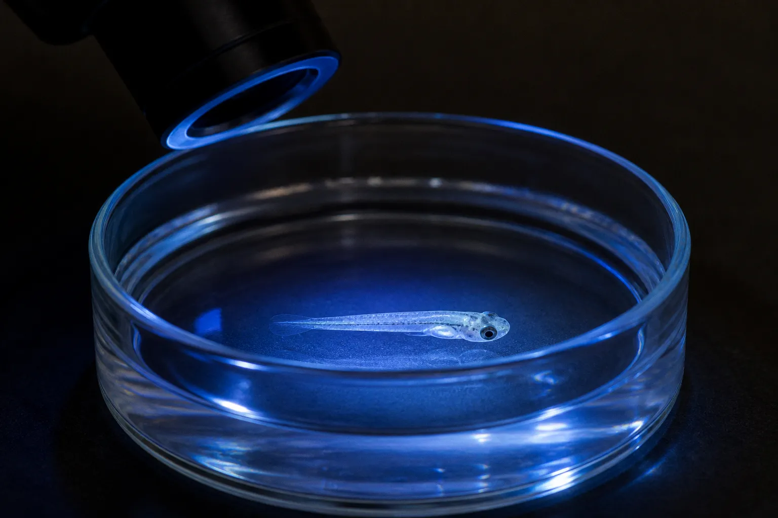
Often, the transgenic line does not match the question: a slow calcium indicator for fast motor dynamics, cytoplasmic expression in a crowded neuropil, or a broad neuronal promoter when you really needed cell-type or tissue-specific signal.
Compare car rental deals in United Kingdom
See available offersPartner link — DiscoverCars comparisonChoosing among transgenic zebrafish lines for calcium imaging is therefore less about finding the “best” GCaMP and more about matching four things: the speed of the biology, the structure you need to segment, the developmental window, and the amount of optical noise your assay can tolerate. Let’s make that choice at the bench level, where it belongs.
Start with the neural event, not the name of the indicator
The GCaMP6s versus GCaMP6f zebrafish comparison gets treated as if one sensor must win. It does not work that way. These variants trade temporal speed for sensitivity, and the right trade depends on whether your experiment is trying to detect small calcium changes or resolve rapidly changing neural activity.
GCaMP6s is the slower, more sensitive option. For a single spike, its approximate time to peak is 179 ms, with a decay time around 550 ms. That extended signal gives small or brief calcium changes more opportunity to rise above the background. It also makes the signal easier to capture when your acquisition rate, photon budget, or preparation is less than heroic—which, on a real imaging day, is most days.
GCaMP6f moves faster: approximately 45 ms to peak and 142 ms decay for a single spike. That makes it better suited to rapidly changing neural dynamics, particularly when you care about the timing between activity and behavior rather than simply whether a neuron became active during a trial.
The practical distinction looks like this:
| Experimental priority | GCaMP6s | GCaMP6f |
|---|---|---|
| Small calcium changes | Strong choice because the slower response supports sensitivity | More likely to trade some sensitivity for speed |
| Fast neural dynamics | Can blur closely spaced events through its longer decay | Better suited to resolving rapid changes |
| Whole-brain activity maps | Useful when detecting broad, low-amplitude responses matters | Useful when temporal precision matters |
| Low-light or photon-limited imaging | Often more forgiving | May require cleaner optics and stronger signal |
| Interpreting event timing | Long decay can make events overlap | Shorter decay reduces temporal smearing |
| Behavioral assays with rapid transitions | May compress several neural events into one prolonged signal | Better for tracking activity around quick sensorimotor changes |
This table is not a substitute for a pilot dataset. It is the decision you should make before the pilot, so the pilot can answer a biological question instead of merely confirming that the camera records green pixels.
Pick the sensor that matches the timescale of the biology. A brighter, slower signal is not automatically a better answer if your question lives in the gaps between events.
When GCaMP6s is the cleaner signal
Choose a slow indicator when your assay focuses on low-amplitude responses, distributed activity, or broad state changes. For example, if you are comparing whole-brain responses to sensory stimulation and the main question is which regions participate, GCaMP6s can give you a useful signal with enough persistence to support registration and segmentation.
That persistence can also help when you are working with a demanding preparation. In larval zebrafish, mounting, immobilization, anesthesia, illumination, and developmental variability all add noise. A sensor with a longer response can be more forgiving when the biological signal is modest.
But the same feature can become a problem. A 550 ms decay is not a neutral detail. If your animal makes rapid turns, escape-like movements, or repeated sensorimotor responses close together, the fluorescence traces may stack on top of one another. You might then interpret one extended calcium transient as a sustained neural state when it actually represents several events.
This is where your analysis choices matter. If you use GCaMP6s for fast behavior, do not quietly treat every fluorescence peak as a timestamp. Align activity to behavior, inspect the raw traces, and test whether the indicator’s decay could merge neighboring events. The sensor is reporting calcium kinetics, not handing you a perfect action potential counter.
When GCaMP6f earns its place
GCaMP6f makes more sense when timing is central: response onset, latency, event order, or the relationship between neural activity and a fast larval movement. Its approximate 45 ms time to peak and 142 ms decay give you a better chance of separating nearby events than GCaMP6s.
That does not mean the fast sensor automatically produces a cleaner movie. Faster kinetics can expose weaknesses in the rest of your prep. If your illumination is uneven, your frame rate is too low, or the expression level varies heavily between animals, the extra temporal performance will not rescue the experiment. You will simply have faster fluctuations in a less reliable signal.
Let’s use a simple what-if.
What if your larval zebrafish turns within a few hundred milliseconds of a visual stimulus?
If you want to know whether a hindbrain population activates before the turn, GCaMP6f is the more defensible starting point. If you only want to map which brain regions respond during the stimulus period, GCaMP6s may give you a more robust regional signal.
What if your stimulus lasts several seconds and produces modest activity across many cells?
GCaMP6s may be the better fit. The longer response supports detection, provided you do not mistake persistence for repeated event timing.
Localization decides whether a neuron is a neuron—or a glowing neighborhood
The second major choice in choosing zebrafish transgenic models is not kinetics at all. It is where the indicator sits inside the cell.
Cytoplasmic GCaMP can produce strong fluorescence, but in the larval zebrafish brain, dense dendrites and axons create a crowded neuropil. With one-photon imaging especially, fluorescence from nearby processes can bleed into a cell-body measurement. That contamination can create apparent correlations between neurons that are not truly sharing activity.
This is the kind of noise that looks biologically interesting. It gives you smooth traces, correlated populations, and a tidy heat map. Unfortunately, tidy is not the same as true.
Nuclear-localized GCaMP for whole-brain segmentation
The line Tg(elavl3:H2B-GCaMP6s) attaches GCaMP6s to histone H2B, restricting the indicator to the nucleus. The elavl3 promoter provides pan-neuronal expression, while nuclear localization reduces signal overlap from surrounding neurites.
For whole-brain functional imaging, this arrangement solves a very practical problem: identifying individual cells. When the signal occupies a compact nuclear region rather than spreading through dendrites and axons, automated or semi-automated segmentation becomes much less of a wrestling match.
That makes H2B-GCaMP6s especially attractive when your priorities include:
- counting active neurons across large brain volumes;
- registering activity to an anatomical reference;
- comparing the same regions across animals;
- reducing overlap in densely packed neuronal areas;
- building cell-by-cell activity maps from light-sheet or other volumetric imaging.
There is a trade-off, and we should say it plainly. Nuclear GCaMP is excellent for locating cell bodies, but it does not give you dendritic or axonal calcium resolution. If your biological question concerns subcellular propagation, synaptic compartments, or process-specific activity, H2B localization has placed the signal in the wrong neighborhood by design.
Use it when the nucleus is the unit you want to measure. Do not choose it and then complain that the dendrites declined to appear.
Soma-targeted GCaMP for cleaner cellular activity
Soma-targeted indicators occupy a useful middle ground. Tg(elavl3:soma-GCaMP7f), for example, restricts GCaMP expression to within approximately 50 μm of the neuronal cell body. That reduces neuropil crosstalk while retaining a somatic signal rather than forcing expression into the nucleus.
This can be a strong option for one-photon imaging, where out-of-focus fluorescence and neuropil contamination can be particularly troublesome. If your analysis depends on comparing activity between individual neuronal somata, soma-targeting may improve the clean signal more effectively than simply increasing expression.
The distinction between H2B and soma-targeted expression is worth keeping visible:
| Feature | Nuclear-localized H2B-GCaMP | Soma-targeted GCaMP |
|---|---|---|
| Signal location | Nucleus | Cell-body region |
| Segmentation | Very strong for compact cell detection | Strong, with more somatic territory |
| Neuropil contamination | Reduced by excluding neurites | Reduced by limiting signal near the soma |
| Dendrite and axon readout | Not suitable | Not designed for process-specific readout |
| Typical strength | Whole-brain cell mapping | Cleaner somatic activity in optical preparations |
| Main caution | Nuclear signal is not a full-cell readout | The soma-targeting radius still does not make contamination impossible |
A useful rule is to decide what your analysis pipeline needs before you choose the line. If the pipeline starts with nuclei detection and atlas registration, H2B-GCaMP6s is logical. If it starts with somatic regions of interest and activity correlations, soma-targeted GCaMP may give you a better signal-to-noise ratio.
Red-shifted soma-targeted indicators
Green GCaMP remains the workhorse, but red-shifted sensors deserve attention when optical constraints or multiplexing matter. SomaFRCaMPi, a red-shifted soma-targeted indicator, has been reported to reduce erroneous neuronal activity correlations by two- to four-fold in zebrafish and mouse brains, largely by reducing neuropil contamination.
That is not a minor cosmetic improvement. False correlations can reshape your interpretation of a circuit. A noisy cytoplasmic preparation may suggest that several populations act as a coordinated ensemble, when the shared signal actually comes from overlapping processes and scattered fluorescence.
A red-shifted indicator can also help when you need to combine calcium imaging with green fluorescent anatomical markers or other optical tools. The exact configuration still needs testing in your microscope, because excitation, emission collection, camera sensitivity, and tissue depth all have opinions of their own. Microscopes are very committed to having opinions.
Promoters determine when and where your signal appears
The indicator variant tells you how the signal behaves. The promoter determines which cells express it and, just as importantly, when expression becomes useful.
For pan-neuronal imaging in larvae, the elavl3 promoter is a familiar and practical choice. Lines such as Tg(elavl3:H2B-GCaMP6s) and Tg(elavl3:soma-GCaMP7f) allow you to survey neuronal activity across the larval brain rather than restricting the experiment to one tissue or cell class.
That broad expression is valuable for whole-brain imaging, but it is not automatically the right answer for every circuit question. If your experiment asks how lateral-line hair cells respond to mechanical stimulation, pan-neuronal expression adds a great deal of biological scenery without improving the specific measurement.
For that tissue, Tg(myo6b:GCaMP6s-caax) provides membrane-localized GCaMP6s expression in lateral-line hair cells and is optimized for imaging larvae from 3 to 7 days post-fertilization. The membrane localization suits a sensory-cell assay, while the developmental window gives you a defined period for planning imaging, stimulation, and replication.
This is an important habit in transgenic line selection: do not choose a broad line simply because it is available in the facility. Choose the line that makes the measured structure resemble the biological unit in your hypothesis.
Early embryogenesis needs a different promoter logic
If the experiment begins during early embryogenesis, the promoter question becomes even more specific. Tg(βactin2:GCaMP6s) provides stronger maternal activity from cleavage through gastrula stages than Tg(ubi:GCaMP6s), making βactin2 the more appropriate starting point when you need expression during those earliest developmental stages.
Here we should resist a common shortcut. “Ubiquitous” does not mean “equally useful at every time point.” A promoter can be broadly active and still produce a different practical expression profile during cleavage or gastrulation. If your imaging begins before tissue organization settles, promoter timing is part of your experimental design, not a footnote in the line name.
Before you commit to a developmental imaging series, map the actual window you need:
1. Define the first biological event you want to capture. Cleavage-stage activity, gastrulation movements, and later neural patterning do not impose the same expression demands.
2. Match promoter activity to that window. βactin2 may be preferable for very early maternal expression, while a neuronal promoter becomes more useful once neural identity and architecture emerge.
3. Check signal distribution in the exact developmental stage. A line that looks excellent at one stage may be unhelpfully dim, diffuse, or anatomically mismatched at another.
4. Separate expression strength from interpretability. More fluorescence can improve detection, but widespread signal may complicate segmentation and increase background.
We do not have a precise, universal maternal expression value for every promoter combination during the earliest cleavage stages, so avoid pretending that one line delivers a fixed fold-change under every husbandry and imaging condition. Your own staging series will tell you more than a confident sentence in a methods section.
Behavioral validation is part of line selection, not an afterthought
A calcium indicator changes the cells you are trying to measure. Even when the animal looks healthy, you should not assume that transgenic expression has no behavioral effect.
The encouraging news is that longitudinal testing of Tg(elavl3:H2B-GCaMP6s) larvae in a casper mutant background from 7 to 28 days post-fertilization found no major differences in locomotion, habituation, stress, or fear responses compared with wild-type fish. That supports the use of this type of pan-neuronal line for behavioral neuroscience assays.
The wording matters: no major differences, not absolutely zero impact. Minor sensorimotor differences can still appear, and a line validated for one behavioral battery may behave differently under another stimulus, developmental stage, illumination regime, or genetic background.
When you compare transgenic zebrafish lines for calcium imaging, pair the imaging validation with the behavior you actually plan to run. A line can perform well in spontaneous locomotion and still alter a more demanding sensorimotor response. Likewise, a line that works in a 7 dpf assay should not automatically inherit a clean bill of health at 28 dpf or beyond.
A sensible validation set includes:
- baseline locomotion before stimulation;
- habituation across repeated trials;
- the specific sensorimotor response central to your assay;
- stress- or fear-related behavior if your experiment uses aversive stimuli;
- developmental survival and general morphology;
- comparison across the genetic background you will actually image.
Keep the design modest but honest. You do not need to reproduce every behavioral assay ever published. You do need enough controls to know whether your neural signal reflects the experimental manipulation or a sensor-related shift in the animal’s baseline.
A line is not validated because the larva swims. It is validated when the animal behaves normally enough for the question you are asking.
Matching lines to common imaging goals
Let’s turn the trade-offs into practical starting points.
Whole-brain functional imaging
For dense, cell-resolved brain mapping, Tg(elavl3:H2B-GCaMP6s) is a sensible first choice when sensitivity and segmentation matter more than millisecond timing. Nuclear localization helps separate neighboring neurons and reduces the contribution of dense neurites.
If your experiment focuses on rapid activity patterns or short-latency behavior, consider a faster indicator or soma-targeted configuration, but check whether the acquisition rate and photon budget can support that choice. A fast sensor cannot create temporal information your microscope never captured.
One-photon imaging with strong neuropil risk
For one-photon imaging, soma-targeted expression is often attractive because it reduces neuropil contamination around the cell body. Tg(elavl3:soma-GCaMP7f) offers a practical route to cleaner somatic traces, particularly when artifactual correlations threaten the interpretation of network activity.
A red-shifted soma-targeted sensor such as SomaFRCaMPi becomes especially interesting when you need reduced erroneous correlation or want to separate calcium imaging from green anatomical fluorescence.
Fast sensorimotor behavior
For escape-like responses, rapid turns, or experiments where neural-behavioral timing matters, GCaMP6f is the more natural starting point than GCaMP6s. Its faster approximate kinetics—45 ms to peak and 142 ms decay—reduce temporal smearing.
Still, test the full chain: stimulus timing, camera frame rate, synchronization, larval movement, and immobilization. If those components drift by more than the biological latency you are trying to measure, the line will not save the experiment.
Early embryonic calcium dynamics
When imaging begins at cleavage through gastrula stages, Tg(βactin2:GCaMP6s) offers stronger maternal activity than Tg(ubi:GCaMP6s) in that early window. The slower indicator also favors detecting modest calcium changes during a period when the preparation and optical geometry may be changing quickly.
Do not carry this choice forward automatically into later neural imaging. An early embryonic promoter and a pan-neuronal larval line answer different logistical problems.
Lateral-line hair-cell imaging
For lateral-line hair cells in larvae from 3 to 7 dpf, Tg(myo6b:GCaMP6s-caax) gives tissue-specific, membrane-localized expression. This is much more useful than imaging a whole-brain line and then trying to excavate the relevant sensory cells from a mountain of unrelated neuronal signal.
The broader lesson applies beyond this one tissue: if your experiment has a sharply defined cellular target, tissue-specific expression can improve both signal interpretation and experimental efficiency.
What about GCaMP7 and GCaMP8?
Newer GCaMP variants may offer meaningful improvements in sensitivity, speed, or dynamic range, and lines such as soma-targeted GCaMP7f are already useful in zebrafish imaging. But choosing the newest name on the list is not a protocol.
For jGCaMP8s or jGCaMP8f, the long-term physiological effects of expression across the entire zebrafish lifespan remain an open question. That does not make these sensors unusable. It means you should separate three claims:
- the sensor can produce a measurable calcium signal;
- the line performs well in your imaging configuration;
- the transgene has no meaningful effect on behavior or physiology across your full study window.
Only the first two may be established in your hands. The third requires validation.
When evaluating a newer sensor, compare it against a line you already understand. Use the same developmental stage, mounting conditions, illumination, acquisition settings, segmentation strategy, and behavioral assay. Otherwise, you are comparing entire experimental ecosystems rather than indicators.
For a practical pilot, quantify:
- baseline fluorescence and background;
- event amplitude and decay;
- the fraction of cells with usable traces;
- segmentation success;
- apparent pairwise correlations;
- motion sensitivity;
- behavioral performance in the same animals or matched siblings.
That dataset will tell you whether the newer line improves your actual assay rather than merely winning a specification sheet contest.
A bench-level decision path
If you are choosing a line this week, start with the biological question and walk through the following sequence:
1. Do you need timing or detection?
For rapid neural events, begin with GCaMP6f or another fast configuration. For small, distributed, or slower responses, GCaMP6s may provide the cleaner signal.
2. What is your unit of analysis?
If you need nuclei for whole-brain cell registration, H2B localization is compelling. If you need somatic activity with less neuropil contamination, use a soma-targeted design.
3. Is the target tissue specific?
Use pan-neuronal elavl3 expression for broad neural surveys, but choose a tissue-specific promoter such as myo6b when a defined sensory structure is the real target.
4. When does expression need to begin?
For cleavage-to-gastrula imaging, βactin2-driven expression may be more suitable than ubiquitin-driven expression. For later larval neural imaging, promoter timing and cellular specificity become more important.
5. Will the optical setup punish diffuse fluorescence?
One-photon imaging and dense neuropil make localization especially important. A soma-targeted or nuclear line may outperform a brighter but more diffuse cytoplasmic signal.
6. Can you validate behavior in the same experimental context?
Include the behavior that anchors your biological conclusion. A line validated for locomotion is not automatically validated for fear, habituation, or a high-speed sensorimotor assay.
The best line is the one that leaves fewer caveats in your conclusion
There is no universal winner among zebrafish calcium indicators. GCaMP6s gives you sensitivity and persistence; GCaMP6f gives you speed. H2B localization makes whole-brain segmentation cleaner; soma-targeting reduces neuropil contamination while preserving a broader somatic signal. βactin2 can support very early embryonic expression, while elavl3 suits pan-neuronal larval imaging and myo6b narrows the field to lateral-line hair cells.
The right choice is the one that makes your final interpretation easier to defend. If your conclusion depends on single-cell identities, do not tolerate avoidable neuropil noise. If it depends on response latency, do not let a slow decay turn several events into one. If it depends on normal behavior, build the behavioral control into the experiment before the first imaging session—not after the figures start looking exciting.
Let’s keep the ambition, but clean up the signal first. Pick the line that matches the biology, run a small side-by-side prep, and make the microscope earn its keep.