Zebrafish brain registration: a guide to Z-Brain mapping
A confocal stack can look perfect and still be analytically unusable. Fluorescent reporters are firing across the optic tectum, the habenula, and the hindbrain; the signal is bright, the volume is clean, and the anatomy is visible.
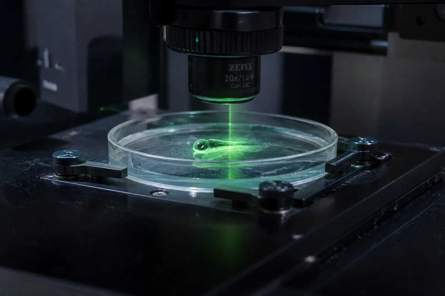
Then you compare it with the next fish and discover that nothing sits in quite the same place. The brain curved differently during mounting. The larva developed at a slightly different pace. Your carefully acquired 3D volume has become an island.
Z-Brain provides the common coordinate system that turns those islands into comparable data. Built from 899 individual brain scans of 6 dpf Nacre/mitfa mutant larvae, the atlas divides the larval zebrafish brain into 294 anatomically defined regions and overlays them with 29 molecular and anatomical labels. Register a new dataset to that reference space with ANTs SyN and the resulting alignment can approach approximately 8 μm—roughly the diameter of a single cell. That is not subcellular precision. It is approximately one-cell-diameter alignment precision, and it sets a realistic upper boundary for claims about spatial localization.
The useful way to think about the zebrafish brain registration Z-Brain atlas protocol is not as a single software command. It is a chain of decisions: developmental stage, pigment background, mounting geometry, acquisition settings, resampling, transform selection, and atlas interpretation. If the early choices are inconsistent, no nonlinear registration algorithm can reconstruct information that was never captured.
Standardizing the 6 dpf Larval Reference Space
The Z-Brain atlas is a 3D digital framework calibrated to a specific developmental moment: six days post-fertilization. Its structural reference channel is based on anti-ERK staining, usually described as total ERK or tERK. That signal is useful because it provides broad brain-wide anatomical contrast without depending on the expression pattern of a particular transgenic reporter.
The age specification is not decorative metadata. At 6 dpf, the major anatomical divisions of the larval brain—the telencephalon, diencephalon, mesencephalon, and rhombencephalon—are sufficiently established to distinguish in a whole-brain volume. At the same time, the larva remains optically accessible enough for confocal imaging through the dorsal-ventral extent of the brain.
Move too far from that reference point and you introduce two kinds of mismatch. Developmental differences alter the size and shape of regions; optical differences alter the quality of the structural signal. A 5 dpf brain is not simply a smaller version of the atlas brain, and a 7 dpf brain may present different proportions and imaging conditions. Registration can compensate for a degree of biological variation, but it should not be asked to erase a systematic staging difference across an entire experiment.
The pigmentation background matters for the same reason. The Nacre/mitfa mutation removes melanophores, the melanin-containing pigment cells that can interfere with optical access and create uneven background in dorsal regions. The reference scans used to construct the atlas come from this mutant background. If your experimental larvae retain wild-type melanophore pigmentation, the problem is not merely cosmetic: the intensity distribution and visible tissue boundaries may differ from those in the template.
PTU needs to be described precisely here. It inhibits melanin synthesis through the melanogenic pathway; it does not remove pigment-cell lineages. In a Nacre/mitfa background, the mutation already eliminates melanophores, while PTU cannot be treated as a general-purpose way to eliminate iridophores or xanthophores. If PTU is included in the laboratory’s preparation protocol, its role should be understood as suppression of melanin production in cells capable of that pathway, not as a replacement for the genetic background or as a treatment that removes every source of pigmentation.
The atlas contains 294 regions, each represented in a common coordinate space. The additional 29 labels provide molecular and anatomical overlays, including reporter-defined domains, neurotransmitter-related populations, and cytoarchitectonic boundaries. Once a dataset is registered, a voxel is no longer only a point in your microscope’s coordinate system. It can be interpreted in relation to the atlas: which anatomical region contains it, which molecular label overlaps it, and which neighboring structures may explain the observed signal.
Z-Brain is not a generic zebrafish brain map. It is a reference space calibrated to a defined developmental stage, genetic background, and structural channel. The closer your sample is to those conditions, the less work the registration has to invent.
Sample Preparation and Confocal Acquisition Parameters
Registration precision is determined partly before the first image is acquired. Motion, optical distortion, pigmentation, compression, and orientation errors all become part of the volume that the algorithm must interpret. A successful transform can correct a specimen’s position and shape; it cannot reliably restore information lost to severe blur or compensate indefinitely for an incompatible reference.
Preparation variables that affect alignment
Raise larvae according to the protocol used by the laboratory and keep the developmental timing consistent across the experiment. If PTU is part of the preparation, use the established concentration and exposure window consistently rather than changing them between clutches. The important distinction is mechanistic: PTU suppresses melanin synthesis in melanogenic cells. It does not eliminate iridophores or xanthophores, and it should not be described as doing so. The Nacre/mitfa background and PTU therefore represent different interventions, not interchangeable versions of the same one.
Anesthetize larvae with Tricaine (MS-222) before mounting and confirm that the animal no longer responds reflexively to a gentle tail touch. The exact working concentration should follow the laboratory’s validated protocol. For registration, the practical endpoint is not a nominal exposure time but a motion-free acquisition. A larva that moves once during a z-stack can produce a discontinuity or blur that later appears as a registration failure.
Mount the specimen in 2.5% low-melting-point agarose, allowing the agarose to cool to approximately 37–38°C before immersion. Excessively warm agarose risks damaging the sample; agarose that is too cool may begin setting before the larva is positioned. Place the larva dorsal-side up in a glass-bottom dish and check its orientation under a stereomicroscope before the matrix sets.
Sagittal alignment is especially important. A small tilt does not automatically invalidate a dataset, but it increases the amount of rotation and asymmetric deformation required during registration. It can also make tissue boundaries appear different across the volume, particularly when the sample is slightly compressed or curved. The aim is a reproducible orientation, not a visually perfect specimen at any cost. If the animal is visibly twisted, it is usually more efficient to remount than to expect the transform to solve the problem later.
| Preparation step | Practical parameter | What it protects against |
|---|---|---|
| Genetic background | Nacre/mitfa mutant reference background | Mismatch in melanophore-associated optical contrast |
| PTU treatment | Use the laboratory’s validated concentration and timing | Melanin-related optical interference in melanogenic cells |
| Anesthesia | Tricaine, with loss of tail-reflex response before mounting | Motion blur and discontinuities through the z-stack |
| Agarose | 2.5% low-melting-point agarose | Drift, movement, or excessive compression |
| Mounting orientation | Dorsal-up, as close to sagittal alignment as practical | Unnecessary rotation and asymmetric deformation |
| Developmental stage | 6 dpf reference stage | Systematic anatomical and optical mismatch |
The point is not to create a perfectly standardized animal. Biological variation remains. The point is to keep technical variation from dominating it. A consistent preparation makes the deformation field biologically interpretable rather than a record of how differently each larva happened to be mounted.
Acquisition geometry
For whole-brain imaging, acquire the complete volume from the dorsal surface to the ventral surface and from the nose toward the spinal cord. The reference acquisition is described at 0.798 × 0.798 × 2 μm. That anisotropic sampling reflects the practical limits of confocal imaging while retaining fine lateral detail and sufficient axial coverage for the full brain.
The structural reference channel should be collected with enough signal-to-noise ratio to show the broad anatomy continuously. Registration does not require every experimental reporter to be bright, because the transform is calculated from the structural channel and then transferred to the other channels. It does require the structural channel to contain recognizable tissue contrast across the volume. A weak or uneven tERK channel makes the algorithm optimize against noise and local intensity artifacts.
Keep the experimental channels in the same spatial frame as the structural channel during acquisition. Calcium indicators, transgenic reporters, activity markers, and immunostains can be separated later, but their voxel geometry must remain compatible with the reference stack. Record the voxel dimensions, image orientation, objective information, and any scaling applied by the microscope software.
Before registration, resample the data to 2 μm isotropic resolution. This reduces the computational burden while retaining the scale required for whole-brain deformation. Feeding the algorithm a much finer volume increases processing time and memory use without turning an atlas-based population registration into a subcellular method. Conversely, downsampling too aggressively removes the anatomical detail needed to match small structures and boundaries.
Multi-channel stacks should be split before entering the registration workflow. In Fiji, separate the tERK structural channel from the experimental signal and export each channel as NRRD or NIfTI. These formats can preserve voxel dimensions, orientation, and other spatial metadata. A file that looks correct when opened but has lost its calibration is not a harmless formatting problem: the registration software will be operating in the wrong physical coordinate system.
Transitioning from CMTK to ANTs SyN for Superior Alignment
The original Z-Brain atlas was constructed with B-spline elastic transformations in the Computational Morphometry Toolkit, or CMTK. That history still matters. Published datasets and older laboratory pipelines may use CMTK, and a legacy result cannot always be regenerated immediately with a different tool.
For new datasets, however, ANTs SyN is the more appropriate choice when the goal is precise nonlinear alignment. SyN—symmetric diffeomorphic normalization—models a smooth, invertible deformation between the sample and the reference. In practice, it is better suited to handling the distributed differences in size and shape that appear across larval brains while preserving a meaningful relationship between neighboring tissue points.
The advantage is not that SyN makes the biology identical. It produces a more coherent mapping of that biological variation into the common atlas space. That distinction matters when the downstream question concerns regional activity, reporter expression, or the relationship between a cell population and a nearby anatomical boundary.
CMTK’s B-spline approach remains usable, particularly when reproducing historical analyses, but it can be less reliable at complex tissue boundaries and small regional transitions. SyN generally offers stronger morphology preservation for new whole-brain registration workflows. The improvement should be assessed on representative samples rather than assumed from a software label alone: inspect the optic tectum, habenula, hindbrain, ventricular contours, and other boundaries where local misalignment becomes obvious.
| Metric | CMTK with B-spline transformation | ANTs with SyN |
|---|---|---|
| Deformation model | B-spline elastic transformation | Symmetric diffeomorphic normalization |
| Typical use | Reproducing legacy atlas workflows | New datasets requiring nonlinear alignment |
| Boundary behavior | Can soften or distort local tissue transitions | Usually preserves anatomical relationships more faithfully |
| Alignment precision | Depends strongly on dataset and parameters | Approximately 8 μm in the described reference workflow—roughly one cell diameter |
| Spatial claim supported | Regional and anatomical comparison | Regional and approximately cellular-scale localization, not subcellular mapping |
| Processing time at 2 μm isotropic input | Pipeline-dependent | Approximately 1–2 hours, depending on hardware and settings |
The approximately 8 μm figure deserves careful language. A distance on the order of 8 μm is comparable to the diameter of a single cell in this context. It is not evidence of subcellular registration. A registered signal that appears within one cell diameter of an atlas boundary may support a cellular-scale interpretation, but it does not establish the position of a nucleus, synapse, membrane compartment, or intracellular structure. The atlas is population-based, and biological variation between individual larvae remains part of the error budget.
If a laboratory has a CMTK pipeline that cannot yet be retired, a useful transition strategy is to process a subset of matched samples with both tools. Compare overlays at region boundaries rather than relying only on a global similarity score. The side-by-side inspection should include the structural reference itself and the transformed experimental channels. A transform that looks numerically acceptable but displaces a narrow anatomical structure can still produce a misleading biological conclusion.
Eight micrometres is a strong whole-brain alignment result when it is measured honestly. It is approximately one cell diameter—not a license to describe an atlas registration as subcellular.
Computational Workflow: From Raw Stacks to Registered Data
The workflow is straightforward in sequence, but each step has a specific purpose. The structural channel drives the transform; the experimental channels inherit it. Do not calculate separate deformations for each reporter unless the analysis specifically requires a different registration strategy, because independent transforms can place channels from the same brain into subtly inconsistent locations.
1. Acquire the full structural volume
Collect confocal z-stacks at approximately 0.798 × 0.798 × 2 μm. Cover the entire brain from dorsal to ventral and from the anterior nose region through the posterior connection toward the spinal cord. Confirm that the field of view does not clip the edges of the brain. A missing dorsal or posterior segment can make the global optimization less stable and will leave no reliable information for the transform to recover.
2. Separate and document the channels
Split the stack into the anti-ERK/tERK structural channel and the experimental channels. Keep a record of which file corresponds to which original channel and verify that all exports retain the same dimensions and orientation. NRRD and NIfTI are suitable working formats because they can carry physical voxel spacing and orientation information more explicitly than a simple image export.
At this stage, inspect the structural channel independently. Look for abrupt intensity changes, saturated areas, empty slices, or motion-related discontinuities. Correcting an acquisition problem before registration is preferable to hiding it with aggressive preprocessing.
3. Resample to 2 μm isotropic voxels
Downsample the volume so that the voxel size is 2 μm in all three axes. Use interpolation appropriate to continuous intensity data for the structural image; bilinear interpolation is one practical option in Fiji for the described workflow. Apply the same geometric resampling logic to the experimental channels so that they remain spatially matched, even if only the structural channel is used to estimate the deformation.
Do not confuse resampling with improved resolution. The 2 μm isotropic volume is a computational representation of the acquired data. It makes the axes comparable and reduces the number of voxels the registration must process. It does not create new optical information.
4. Register the structural channel to the atlas
Use the tERK template from Z-Brain as the fixed image and the sample’s structural tERK channel as the moving image. ANTs SyN then estimates the transformations needed to bring the sample into reference space. The output includes a deformation field and an inverse transform, allowing movement between sample coordinates and atlas coordinates.
The exact parameter schedule should be validated against the microscope, preprocessing choices, and computing environment. A command that works on one batch may fail on another if intensity ranges, cropping, or metadata differ. Monitor the output visually. The transformed tERK image should follow the major contours of the atlas without implausible folding, tearing, or local stretching.
5. Apply the same transform to experimental data
Use antsApplyTransforms or the equivalent application step to move the calcium, reporter, activity, or immunostaining channel into Z-Brain space. The transform must be applied with interpolation suitable for the type of data. Continuous fluorescence intensity and discrete region masks should not automatically be treated the same way: interpolating a label map as if it were a continuous signal can create artificial intermediate values at boundaries.
The transformed experimental channel is now comparable across animals. It can be overlaid on the atlas template, inspected against regional masks, and analyzed alongside other registered samples. Keep the original, unregistered data as the primary record. Atlas-space images are derived products, not replacements for the raw acquisition.
6. Query the anatomical masks
Each of the 294 regions can be represented by a corresponding mask. Apply those masks to the registered experimental channel to calculate regional signal, expression, activity, or labeling intensity. This is where a coordinate transform becomes a biological measurement: the analysis changes from “bright pixels in this part of the image” to a defined signal distribution across named anatomical regions.
The full path from raw stack to region-level quantification can take approximately 2–3 hours per brain on standard computational hardware, with the main cost usually concentrated in the ANTs registration step. Processing time will vary with the number of voxels, memory, CPU configuration, preprocessing, and parameter schedule. The useful benchmark is not the fastest runtime but the reproducibility of the transform and the stability of the regional measurements.
Navigating the 294 Anatomical Regions and Molecular Labels
Atlas registration is only valuable if the atlas labels are used with the same care as the transform. A registered image is not automatically a correct anatomical interpretation. The 294 regions span the larval brain and are organized across its major divisions:
- Telencephalon: including the olfactory bulb, pallium, and subpallium.
- Diencephalon: including the habenula, thalamus, hypothalamus, and pretectum.
- Mesencephalon: including the optic tectum and tegmentum.
- Rhombencephalon: including the cerebellum, hindbrain reticular formation, and motor nuclei.
The molecular and anatomical labels add a second layer. They may identify neurotransmitter-related systems, transgenic reporter domains, and cytoarchitectonic landmarks that do not correspond one-to-one with the 294 anatomical regions. A signal can therefore overlap an anatomical mask and a molecular label at the same time. Those overlaps are useful, but they should not be presented as if every label were an independent, perfectly bounded structure.
For example, “signal in the optic tectum” is a broad regional statement. A more informative analysis may ask whether the signal is concentrated in a particular tectal layer, near a defined molecular domain, or adjacent to a neurotransmitter-associated population. The answer depends on registration quality, the spatial scale of the original signal, and the resolution of the atlas label. If the signal is diffuse or the boundary is uncertain, report that uncertainty rather than converting a visual impression into a precise cellular claim.
Whole-brain activity mapping
The MAP-Mapping assay—Mitogen Activated Protein kinase Mapping—uses the ERK pathway to estimate neural activity across the brain. In a typical workflow, phosphorylated ERK is measured relative to total ERK before fixation and registration. The pERK-to-tERK relationship provides an activity-related signal that can then be placed into Z-Brain space.
The atlas makes that measurement anatomically useful. Instead of producing a whole-brain intensity image with no common coordinate system, the registered activity data can be compared across larvae and summarized by anatomical region. The resulting analysis may distinguish activity in the hindbrain from activity in the optic tectum, or separate a broad diencephalic pattern from a more localized habenular signal.
The same caution applies here as to reporter imaging: atlas registration improves comparability, but it does not eliminate biological variability. A region-level activity difference is strongest when the acquisition, staging, preprocessing, and normalization are consistent across all samples. If one group was mounted differently or imaged with a weaker structural reference, the apparent biological difference may partly reflect the registration pipeline.
Region masks and quantitative summaries
When extracting signal with a region mask, decide in advance how to handle edge voxels, background, and overlapping labels. Mean intensity, integrated intensity, positive-volume fraction, and normalized activity ratios answer different questions. A mean can hide a small, bright population; integrated intensity can be affected by region volume; and a positive-volume metric depends on the thresholding method.
Do not treat a mask as a substitute for visual quality control. Overlay the mask on the transformed structural and experimental channels. Check whether the signal is plausibly located within the region and whether it is being clipped at the edge of the volume. A technically valid multiplication of an image by a mask can still produce a biologically meaningless result if the deformation has displaced the relevant structure.
Troubleshooting the Registration Pipeline
Most failures can be traced to a mismatch introduced before or during transformation. The solution is usually to identify the stage at which the mismatch entered rather than to increase every registration parameter at once.
Pigmentation or uneven background in dorsal imaging. First distinguish the genetic background from the PTU protocol. Nacre/mitfa removes melanophores; PTU inhibits melanin synthesis in melanogenic cells and does not remove iridophores or xanthophores. If the sample has optical interference, verify the line, staging, treatment history, and structural-channel quality instead of describing PTU as a universal pigment-cell elimination step.
Asymmetric warping after registration. Reinspect the mounting geometry. A larva that was tilted, twisted, or compressed before the agarose set may require a large deformation that distorts local boundaries. Compare the raw tERK volume with the atlas before checking the experimental channel. If the structural anatomy is already implausible after transformation, the reporter is not the primary problem.
Failure to converge. Check the image dimensions, physical voxel spacing, orientation, and intensity range. A file can retain the correct visual appearance while losing the metadata that tells ANTs how large each voxel is. Also confirm that the structural channel covers the full brain and that resampling produced 2 μm isotropic data rather than merely changing the displayed scale.
Blur in the registered image. Registration does not cause every form of blur. Motion during acquisition, sample drift, poor signal-to-noise ratio, and interpolation during repeated resampling are common causes. Keep the number of resampling operations low and apply the final transform directly to the original channel where practical.
Misalignment at tissue boundaries. Compare ANTs SyN with the historical CMTK workflow on the same sample if the discrepancy is unclear. Inspect local anatomy, not only a whole-volume similarity score. If CMTK is required for an existing dataset, document that constraint and avoid presenting its output as directly interchangeable with a newly generated SyN result without validation.
Overinterpretation of a successful transform. Even a visually strong alignment does not support subcellular localization. The approximately 8 μm precision described for the workflow is about one cell diameter. It can support regional comparisons and, under favorable conditions, approximately cellular-scale localization. It cannot establish the position of a synapse, a subcellular compartment, or a boundary with certainty below that scale.
Biological variation also places a limit on what an atlas can do. Individual larvae differ in brain size, shape, developmental timing, and labeling intensity. A population-averaged reference is designed to make those samples comparable, not to make them identical. If the experiment requires spatial information finer than the atlas can support, the appropriate response is a different experimental design—such as internal landmarks or single-animal longitudinal imaging—not a more aggressive deformation field.
Before the First Registration
A reliable run begins with a short parameter review, but the review should be treated as part of the experimental record rather than as a generic checklist. Confirm that the larvae match the intended Nacre/mitfa reference background and that the developmental stage is 6 dpf. Record whether PTU was used, at what stage, and for what purpose; keep its action described accurately as inhibition of melanin synthesis rather than elimination of pigment-cell populations.
Before mounting, verify the anesthesia endpoint and prepare 2.5% low-melting-point agarose at an appropriate temperature. Place the larva dorsal-side up and check sagittal alignment before the agarose sets. During acquisition, collect the complete brain at approximately 0.798 × 0.798 × 2 μm and preserve the same field geometry across animals.
After acquisition, split the channels without losing spatial metadata. Export the structural and experimental images as NRRD or NIfTI, resample to 2 μm isotropic resolution, and use the tERK channel—not the activity reporter—as the moving image for registration. Register the sample to the Z-Brain template with ANTs SyN, then apply the resulting deformation field to every experimental channel that must remain spatially matched.
Finally, inspect the transformed structural image before extracting regional values. Apply the 294-region masks only after the anatomy is plausibly aligned, and keep the original data alongside the atlas-space derivatives. This preserves the distinction between what the microscope measured, what the registration estimated, and what the atlas allowed you to name.
The power of Z-Brain is not that it removes variation from zebrafish neurobiology. It gives that variation a shared coordinate system. When staging, preparation, acquisition, and computational transforms are controlled, a whole-brain volume can be compared with the next animal, the next experiment, and the next perturbation. The result is not subcellular certainty. It is something more useful and more defensible: approximately one-cell-diameter alignment across a defined larval reference space, connected to 294 anatomical regions and a set of molecular labels that make whole-brain imaging interpretable.