Spinal cord circuit mapping in larval zebrafish
You have a spinal cord roughly 300 microns wide. It contains hundreds of interneuron subtypes making thousands of synaptic contacts onto a compact motor column.
The Mapping Problem
You need to know which cells connect to which — and how those connections assemble as the system comes online. The brute-force approach — slice, stain, image, repeat — gets you nowhere at the resolution that matters. What you need is a toolkit that resolves individual synaptic contacts in intact tissue, at speed, across entire cell populations.
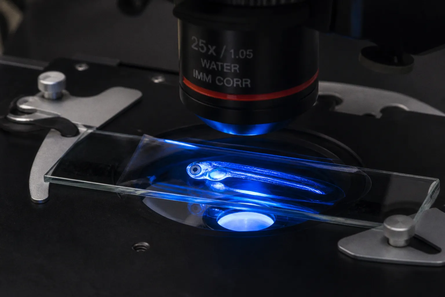
Larval zebrafish offer a narrow but powerful window. By 3–5 days post-fertilization (dpf), the spinal cord is functionally active, optically transparent, and genetically accessible. The animal swims. The circuits fire. And the tissue stays thin enough for photon-based interrogation at cellular resolution. That combination — optical clarity, genetic tractability, and functional readiness — is what makes this model the workhorse for synaptic connectivity mapping at scale.
But "workhorse" does not mean "easy." Each method in the zebrafish spinal cord toolkit trades off specificity against throughput, spatial resolution against temporal dynamics, and synaptic proximity against circuit breadth. Knowing which assay answers which question — and where each one breaks — is the difference between clean data and noise dressed up in fluorescent colors.
This guide walks through the core methods, their operating parameters, and their failure modes. It is structured for the practitioner who needs to build a mapping pipeline, not for the reader who wants a review of the field.
Optical and Genetic Tools for Synaptic Labeling: GRASP and Trans-Tango
The fundamental challenge in circuit mapping is proximity. Two neurites can be microns apart and share zero synaptic contacts. Conventional fluorescence colocalization cannot distinguish a synapse from a near-miss. You need a signal that only fires when a molecular interaction occurs at the synaptic cleft itself.
GRASP (GFP Reconstitution Across Synaptic Partners) solves this with a split-reporter architecture. Each half of a GFP variant is tethered to the extracellular surface of either the presynaptic or postsynaptic membrane. When a synapse forms, the two halves are close enough to refold into a fluorescent molecule. The signal is binary and spatially precise: no synapse, no light.
In larval zebrafish, GRASP has been optimized specifically for mapping premotor inhibitory inputs onto motor neurons. The dmrt3a-labeled dI6 interneurons — a critical class of spinal interneurons that gate left-right alternation — have been mapped using this approach. The readout is clean. You see a punctate signal at the contact interface, and you can quantify it against background across the entire motor column.
The limitation is static. GRASP reports a cumulative history of synaptic contacts, not their real-time dynamics. It tells you "these cells formed synapses," not "these cells are talking right now." For developmental mapping — establishing the wiring diagram — that is sufficient. For functional interrogation, you need a different tool.
Trans-Tango brings a transsynaptic signal transfer that is genetically encoded. The system places a ligand (hGCG fused to neurexin 1a or 1b and ICAM1) on the presynaptic membrane and a receptor (hGCGR fused to a QF transcription factor via a TEV protease cleavage site) on the postsynaptic membrane. When a synapse forms, the ligand activates the receptor, cleaving the transcription factor into the postsynaptic nucleus. The result: a reporter gene turns on exclusively in cells that receive synaptic input from a defined population.
The adaptation of trans-Tango to zebrafish, reported in 2023, expanded the genetic toolkit considerably. You can now label postsynaptic targets of a genetically defined presynaptic population without relying on split-fluorescence reconstitution. The readout is nuclear, which simplifies segmentation. The signal amplifies through transcription, which improves sensitivity.
The shift from GRASP to trans-Tango is not a replacement — it is a complementary axis. GRASP maps synaptic contact sites. Trans-Tango maps synaptic partners. They answer different questions about the same circuit.
Neither method resolves synaptic dynamics. Neither tells you signal polarity or strength. For that, you move to optogenetic interrogation.
High-Throughput Connectivity: Combining Two-Photon Optogenetics and Calcium Imaging
The fastest route from "which cells connect" to "what does the connection do" is simultaneous presynaptic stimulation and postsynaptic recording. In a system as compact as the larval zebrafish spinal cord, two-photon optogenetics paired with volumetric calcium imaging gets you there at single-cell resolution.
The protocol in brief: express a soma-targeted opsin (CoChR-EGFP-Kv2.1) in your presynaptic population. Express a red calcium indicator (jRGECO1b) broadly across the spinal cord. Use a two-photon laser at 950 nm to activate individual somata while simultaneously recording calcium transients in surrounding cells.
The spatial resolution numbers matter here. The system achieves approximately 6 microns lateral and 12–15 microns axial resolution. The average soma diameter of a larval zebrafish spinal neuron is 6.6 microns. That means lateral stimulation is soma-matched, while axial resolution introduces a small but real risk of collateral activation — photostimulating an adjacent cell body stacked above or below your target.
This is not a trivial concern. At suprathreshold stimulation intensities, the axial blur can recruit unintended cells. The data then carries false-positive connections. Calibration is critical. You titrate laser power to the minimum that reliably drives spikes in your target cell, verified by concurrent whole-cell patch-clamp recording. Only after establishing the threshold do you scale to high-throughput screening mode.
In that screening mode, the system is powerful. You photoactivate one cell at a time across a grid, recording calcium responses across the entire field. Each stimulus is a data point in a connectivity matrix: presynaptic cell × postsynaptic response. Scale that across hundreds of stimulation sites, and you build a dense map of local synaptic connectivity at cellular resolution.
| Parameter | GRASP | Trans-Tango | Two-Photon Opto + Calcium | Rabies Tracing | vEM |
|---|---|---|---|---|---|
| Readout | Fluorescent puncta | Nuclear reporter | Calcium transient | Fluorescent label | 3D ultrastructure |
| Temporal resolution | Static (cumulative) | Static (cumulative) | Milliseconds | Static (cumulative) | Static (fixed tissue) |
| Directionality | Synapse-specific | Input-defined | Excitatory/inhibitory inferred | Retrograde monosynaptic | All contacts, anatomical |
| Throughput | Moderate | Moderate | High | Moderate | Low |
| In vivo | Yes | Yes | Yes | Yes | No (fixed) |
The workflow scales. A single preparation can yield connectivity data for 50–100 presynaptic cells against the full local postsynaptic population. Combined with genetic subtyping of the stimulated population, you can ask: does a dmrt3a+ interneuron connect to a specific motor neuron subtype? The answer comes as a probability, quantified across animals.
Retrograde Tracing and Viral Vector Optimization in Larval Models
If optogenetics maps forward connectivity — who drives whom — then retrograde tracing maps the inverse: who provides input to a defined cell. The gold standard for this is glycoprotein-deleted rabies virus, and the zebrafish field has optimized it substantially.
The system works in two steps. First, you express two components in your starter cell: the EnvA receptor TVA (which restricts viral entry to engineered cells) and the rabies glycoprotein (which enables transsynaptic spread). Second, you apply EnvA-pseudotyped, glycoprotein-deleted rabies virus. It enters only cells expressing TVA. Once inside, it replicates and spreads retrogradely across exactly one synapse, labeling every direct presynaptic input to your starter cell.
The critical optimization in recent zebrafish work involves the CVS strain of rabies virus, trans-complemented with N2cG at 36 degrees Celsius. This temperature step is non-negotiable for efficiency. At standard zebrafish rearing temperatures (28 degrees Celsius), the virus replicates poorly. Bump it to 36 degrees for the incubation period, and tracing efficiency climbs to up to 20 labeled input cells per starter cell.
There is a cytotoxicity constraint. Rabies virus is not benign. It kills cells — just slowly enough that viable imaging is possible up to 10 days post-infection. You design your experiment window around this. Day 3–5 post-infection is the practical sweet spot: signal is strong, cell death has not yet compromised the tissue.
Steps to optimize rabies-based retrograde tracing in your zebrafish spinal cord preparation:
1. Starter cell expression. Drive TVA and glycoprotein from a cell-type-specific promoter. Verify co-expression before virus injection. Poor co-expression means low starter efficiency and wasted animals.
2. Virus titer calibration. Inject serial dilutions. The goal is sparse starter labeling — one to five starter cells per spinal cord. Too many starters, and the monosynaptic restriction degrades.
3. Temperature shift. Transfer injected larvae to 36 degrees Celsius for 12–24 hours, then return to 28 degrees. This window balances viral replication against thermal stress.
4. Imaging window. Fix and image at 4–6 days post-infection. Earlier, and signal is weak. Later, and cytotoxic artifacts accumulate.
5. Controls. Run the virus on animals lacking TVA. Any labeled cells indicate leaky entry and invalidate your dataset.
The rabies virus is a precision instrument with a timer attached. You have roughly a week of usable signal. Design your imaging and analysis pipeline to run within that window, or start over.
Ultrastructural Insights: Volume Electron Microscopy and Wiring Specificity
Every optical method has a resolution ceiling. GRASP and trans-Tango label synapses as dots. They cannot resolve vesicle pools, cleft geometry, or the number of release sites per synapse. For that level of detail, you need electron microscopy — and specifically, volume EM (vEM) that reconstructs tissue in three dimensions across contiguous serial sections.
The 2018 volume EM reconstruction of the larval zebrafish spinal cord was a methodological inflection point. It mapped all synaptic connections from specific interneuron classes onto all motoneurons in a defined spinal segment. The result was not just a connectivity table but a wiring diagram annotated with synapse number, contact area, and position along the postsynaptic dendrite.
What the data showed was wiring specificity that was invisible to light microscopy. Interneurons targeting different motor neuron pools did not just "connect" — they formed synapses at precise subcellular locations, with contact numbers that correlated with the functional role of the circuit. Speed-related motor circuits showed a particular wiring logic: the number and placement of synapses were matched to the temporal demands of the behavior.
The trade-off is throughput. Volume EM of even a single spinal segment takes weeks of imaging and months of reconstruction, whether manual or AI-assisted. You cannot use vEM as a screening tool. You use it to validate and deepen the maps generated by faster methods — to answer the question: when GRASP says two cells are synaptic partners, what does that synapse actually look like?
The practical workflow pairs vEM with optogenetic connectivity data:
- Step 1. Map connectivity at cellular resolution using two-photon optogenetics + calcium imaging.
- Step 2. Identify high-confidence connections and repeat connections across animals.
- Step 3. Target those specific cell pairs for vEM reconstruction.
- Step 4. Quantify synapse number, vesicle content, cleft width, and postsynaptic density area.
This pipeline converts vEM from a fishing expedition into a hypothesis-driven structural assay. You already know what to look for. You are measuring its ultrastructure, not discovering its existence.
Mechanical Dynamics and Regenerative Capacity of the Spinal Cord
Circuits do not exist in a mechanical vacuum. The spinal cord is a soft tissue with specific elastic and viscous properties that change during development and after injury. Understanding those properties matters for two reasons: mechanical forces influence circuit assembly, and mechanical disruption (injury) tests circuit resilience.
Confocal Brillouin microscopy now allows quantitative mapping of the apparent longitudinal modulus and viscosity of spinal cord tissues in living zebrafish larvae. This is a label-free, non-contact technique. You probe the tissue with a focused laser and measure the frequency shift of scattered light, which correlates directly with local stiffness. The result is a spatial map of mechanical properties — across gray matter, white matter, and the central canal — in an intact, living animal.
The zebrafish larva's regenerative capacity adds a second layer. Mechanical transection of the spinal cord at 3 dpf — whether by incision or perforation — is followed by axonal regrowth and functional recovery within two days. Two days. The animal resumes swimming behavior. The circuits reconnect, at least partially.
This regenerative timeline establishes a hard experimental boundary. If you are studying developmental circuit assembly, injury before 3 dpf introduces a confound: the regenerating circuit may wire differently than the intact one. If you are studying regeneration, you must control for developmental stage — the same lesion at 5 dpf yields different regenerative kinetics than at 3 dpf.
The mechanical data from Brillouin microscopy adds nuance here. After injury, the lesion site shows a transient softening — a drop in apparent modulus — that recovers as tissue integrity is restored. That mechanical signature correlates with the window of axonal regrowth. Whether the softening enables regrowth or merely accompanies it is still unresolved. What is clear is that the mechanical environment is not a passive scaffold; it is a variable that the circuit must navigate.
Building Your Pipeline: A Practical Checklist
Every method described above answers a specific question. No single technique covers the full scope of spinal cord circuit mapping. The pipeline you build depends on the question you are asking, the throughput you need, and the resolution you can tolerate.
A working setup for a comprehensive mapping study in larval zebrafish spinal cord:
1. Define your presynaptic population genetically. Use cell-type-specific Gal4 or Cre lines. Without genetic precision, every downstream assay is contaminated with off-target signals.
2. Run GRASP for initial synaptic contact mapping. Get a baseline connectivity table. Identify candidate partners.
3. Confirm with trans-Tango in the reverse direction. If GRASP says cell A synapses onto cell B, trans-Tango from cell B should label cell A as an input. Cross-validation eliminates false positives.
4. Quantify functional connectivity with optogenetics + calcium imaging. Establish the probability and strength of each connection. Titrate stimulation parameters against patch-clamp ground truth.
5. Trace retrograde inputs with rabies virus. Map the full presynaptic ensemble onto your target cell. Respect the 10-day viability window.
6. Validate ultrastructure with targeted vEM. Select your strongest candidate connections from steps 2–5. Measure synapse number and morphology.
7. Assess mechanical context with Brillouin microscopy. Map tissue stiffness across your region of interest. Correlate mechanical gradients with circuit density.
Calibrate. Quantify. Map. The spinal cord yields its wiring logic to the method that asks the right question at the right resolution. Everything else is noise.