Zebrafish axon guidance tracking: a dual-color imaging plan
Axon guidance experiments fail at the same point more often than they fail at the microscope: the signal does not separate the structures that must be mapped. Overlapping arbors collapse into one fluorescent mass.
Pioneer axons disappear behind brighter bundles. A time-lapse sequence records movement, but not the path taken by a defined neuron.
A robust zebrafish axon guidance tracking method starts by assigning the two colors a job. One channel should identify the axon population or reference structure. The second should expose the trajectory, target field, competing arbor, or manipulated cell. If both channels simply label everything, dual-color imaging adds complexity without adding circuit information.
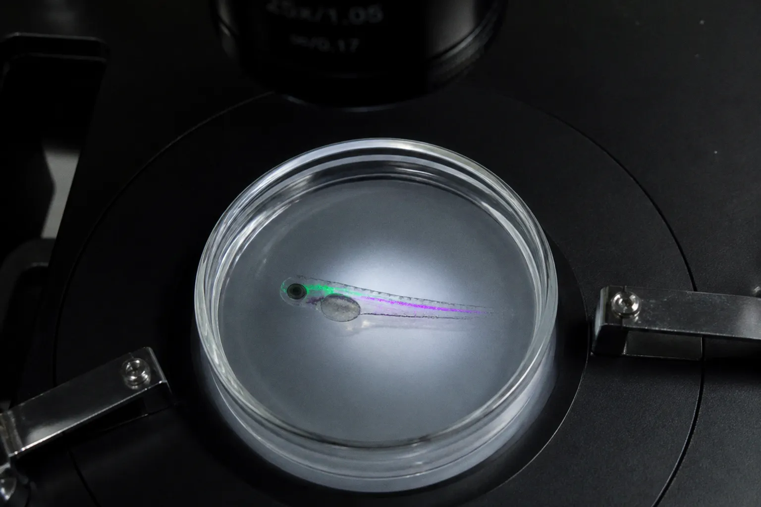
Embryonic zebrafish provide the necessary geometry for this approach. Their transparency allows non-invasive, high-resolution imaging of axon growth in vivo across both the central and peripheral nervous systems. With transgenic fluorescent expression, multispectral labeling, and a calibrated acquisition plan, the experiment can follow individual pioneer axons, quantify path deviations, and connect early growth behavior to later synaptic architecture.
Start with the circuit question, not the fluorophores
The imaging plan should resolve one mechanical problem:
- Which axon establishes the initial route?
- Which guidance cue changes the trajectory?
- Does an axon reach the correct target but stratify incorrectly?
- After axotomy, does the original path re-form?
- Does a manipulated neuron reconnect with the correct partner?
- Are overlapping arbors produced by one lineage or by several cell populations?
These questions require different labels and different endpoints. A two-color scheme for mapping axon pathfinding is not automatically suitable for measuring synaptic connectivity. The first task is to define the observable.
For example, if the objective is to track a pioneer axon, use one channel to isolate that neuron or lineage and the second to mark the surrounding pathway. The reference channel may show a target region, a fascicle, or a neighboring axon class. If the objective is to measure regeneration after targeted injury, the second channel should help locate the lesion and distinguish regrowing segments from intact axons.
The color assignment is secondary. Structural separation comes first.
Dual-color imaging is useful only when each channel answers a different circuit question.
A practical plan contains four layers:
1. Identity — which neuron, lineage, or axon class is being tracked?
2. Geometry — what path, boundary, layer, or target defines correct navigation?
3. Perturbation — what changes the system: axotomy, optogenetic activation, genetic manipulation, or altered development?
4. Quantification — which measurement will distinguish normal guidance from error?
Without the fourth layer, the experiment becomes a sequence of attractive images. That is not circuit analysis.
Build the dual-color architecture
Choose the label strategy
Fluorescent protein expression can be driven in transgenic zebrafish lines using promoter-defined neuronal populations. The first channel may use GFP or CFP. The second may use RFP or YFP. These combinations are familiar, but the relevant criterion is not the name of the protein. It is the separation of emission and excitation signals under the selected microscope configuration.
For dense or overlapping circuits, a simple two-color arrangement may not resolve enough cells. Multispectral approaches such as Zebrabow generate a wider range of fluorescent identities. This adapts the Brainbow principle to zebrafish and can separate overlapping axonal arbors while supporting cell-lineage tracing.
Use multispectral labeling when the circuit contains:
- Several axons with similar trajectories.
- Dense terminal fields.
- Interwoven branches that cannot be assigned by position alone.
- A need to connect a mature arbor to a developmental lineage.
- Repeated branching patterns that make morphology alone ambiguous.
Do not treat Zebrabow as a replacement for experimental design. More colors increase identity information, but they also increase the burden of spectral separation, intensity normalization, and image analysis. If the circuit can be resolved with two clean channels, use two.
Match the microscope to the depth and time scale
Two-photon excitation is suitable when the axon must be tracked inside live tissue at depth. A tuned Ti:Sapphire laser can support separate excitation conditions, such as approximately 850 nm for CFP and approximately 930 nm for RFP or YFP. A water-immersion objective is required for the live preparation. One documented configuration uses a 20× W Plan-Apochromat objective with numerical aperture 1.0.
These parameters are not universal settings. They define a starting architecture. The final excitation range, detector arrangement, gain, and exposure must be calibrated against the fluorophore pair, embryo preparation, optical path, and time-lapse duration.
Light-sheet microscopy becomes useful when the experiment prioritizes low phototoxic burden across a larger volume or when the circuit develops through a three-dimensional field that is difficult to sample with repeated point scanning. Confocal time-lapse imaging remains useful for dynamic tracking and for combining with targeted two-photon axotomy. The selection should follow the measurement:
| Experimental demand | Suitable imaging priority | Main output |
|---|---|---|
| Track a defined axon at depth | Two-photon imaging with separated excitation channels | Axon trajectory and growth dynamics |
| Survey a larger developing volume | Light-sheet imaging | Network-scale assembly and branching |
| Monitor a targeted lesion over time | Two-photon axotomy plus confocal time-lapse | Regeneration and reconnectivity |
| Resolve dense overlapping arbors | Multispectral labeling such as Zebrabow | Cell identity and lineage separation |
| Test local control of growth | Focal activation of photoactivatable proteins | Directional response and path correction |
The table is a planning tool, not a substitute for calibration. A microscope can collect two colors and still produce unusable data if the channels bleed into one another or if one fluorophore saturates before the other becomes visible.
Calibrate the channels before collecting a time series
The first calibration target is cross-talk. Image single-color controls under the planned acquisition conditions. Measure whether the CFP signal appears in the RFP channel or whether the RFP/YFP signal contaminates the CFP channel. The problem becomes harder when the brighter label occupies a larger arbor.
Next, check dynamic range. Keep the brightest structures below saturation while retaining enough signal from thin axonal branches. Saturated pixels erase the very information needed for path tracing: branch points, growth-cone position, and contact with the target field.
Then assess registration. The two channels must remain spatially aligned across the field and through the relevant depth. A small offset can appear as a false separation between an axon and its target. This matters when the endpoint is a contact event rather than a broad anatomical overlap.
Finally, calibrate the time interval. The interval must be short enough to capture meaningful growth changes but long enough to limit photobleaching and phototoxicity. Exact laser-power thresholds for multi-hour imaging depend on the setup and should not be assumed from a generic plan. The correct value must be established empirically for the preparation.
Map axon guidance as a sequence of measurable states
Axon guidance mechanisms in zebrafish are best analyzed as transitions, not as a single final image. A developing axon moves through recognizable states:
1. Emergence — the axon leaves the soma or initial fascicle.
2. Extension — the growth cone advances along a defined route.
3. Decision point — the axon turns, branches, crosses, or selects between pathways.
4. Target entry — the axon reaches the target territory.
5. Arbor formation — terminal branches occupy a specific region or layer.
6. Connectivity — the mature pattern supports a defined synaptic relationship.
The dual-color dataset should preserve these transitions. A final projection may show where the axon ended. It cannot reliably show how it arrived there.
For each tracked axon, record a consistent set of variables:
- Starting position relative to the soma or reference landmark.
- Time of initial extension.
- Direction of the primary trajectory.
- Turning angle at each decision point.
- Number and location of branches.
- Distance from the intended pathway.
- Time of target entry.
- Terminal-field location.
- Persistence or disappearance of the branch.
- Response after perturbation or injury.
The simplest useful measurement is trajectory displacement. Define the expected path using the reference channel, then quantify the distance between the tracked axon and that route over time. A path that eventually reaches the target may still show a prolonged guidance error. That delay can be biologically relevant.
For individual axon tracing, tools such as the NeuronJ plugin in ImageJ can support manual or semi-assisted path reconstruction. The analysis should retain the original image stack, channel assignments, and tracing decisions. Do not reduce the dataset to a single overlay. The overlay is for interpretation. The raw channels are for verification.
Treat the reference channel as geometry
The reference signal should constrain interpretation. It can define a target, a fascicle, a neighboring population, or a layer boundary. Use it to establish a coordinate system.
For a simple pathfinding experiment, map:
- Axon centerline.
- Reference pathway centerline.
- Distance between the two.
- Turning points.
- Endpoint position.
For a layered terminal field, map the depth of arborization relative to the layer boundaries. In retinal circuit work, the inner plexiform layer is divided into sublaminae s1–s6. Those sublaminae provide a defined stratification coordinate rather than a vague description such as shallow or deep. Do not generalize this coordinate system to unrelated circuits. Use it where the anatomy supports it.
A practical output is a trajectory map with each branch assigned to a time point and a spatial compartment. This lets you separate three errors that are often merged:
- Path error: the axon takes the wrong route.
- Targeting error: the axon reaches the wrong region.
- Stratification error: the axon reaches the correct region but occupies the wrong layer.
The same final fluorescent density can result from all three. The time-resolved dual-color record distinguishes them.
Use perturbation to test mechanism
A descriptive movie shows what the axon does. A perturbation tests why it does it.
Targeted axotomy
Two-photon laser axotomy can sever a selected axon in a live zebrafish embryo. Pairing the injury with confocal time-lapse imaging allows the experiment to follow the axonal response in real time.
The dual-color plan should separate:
- The axon selected for injury.
- The surrounding pathway or target structure.
- The proximal and distal segments after the cut.
- New growth from the injured neuron.
- Reconnection with the original route or an alternative route.
The key endpoint is not simply regeneration. Regrowth can occur without correct reconnection. Quantify the new trajectory against the pre-injury path and the reference channel. Record whether the axon re-enters the original fascicle, reaches the target field, and recreates the previous terminal arrangement.
A clean axotomy experiment requires spatial precision. The lesion must be visible in the image stack. The analysis must distinguish a true severed segment from temporary loss of fluorescence caused by movement, bleaching, or focal drift.
Photoactivatable control of axon growth
Focal activation of photoactivatable proteins such as photoactivatable Rac1 can manipulate axonal growth trajectories in live zebrafish embryos. The approach provides local control rather than a whole-animal change in signaling.
Here the color channels should answer two separate questions:
- Where is the axon and how does its growth cone move?
- Where and when was the photoactivatable signal activated?
The activation region must be registered to the axonal trajectory. A response is more credible when the experiment records baseline growth, applies the focal activation, and then quantifies the change in direction or extension rate using the same coordinate system.
Avoid treating a single turn as proof of guidance control. Compare repeated activation events, sham illumination, and non-activated controls where possible. The measurement should capture the directional response rather than rely on visual impression.
Separate assembly from maintenance
Neural network assembly tracking and mature circuit mapping answer different questions. During development, a branch may be transient. In a mature preparation, the same region may appear stable because unstable branches have already been eliminated.
Use time-lapse imaging to characterize assembly:
- When does the axon enter the pathway?
- How long does it remain at a decision point?
- Which branches persist?
- Does the target field stabilize before or after terminal refinement?
Use endpoint imaging to quantify the final architecture:
- Branch density.
- Arbor area.
- Layer occupancy.
- Target overlap.
- Connectivity pattern.
Do not infer developmental mechanism from a single mature snapshot. It can locate the endpoint. It cannot reconstruct the sequence that produced it.
Control the failure modes before interpreting biology
The most common errors are operational. They arise from signal imbalance, motion, spectral contamination, and weak identity assignment.
Signal imbalance
If one fluorophore is substantially brighter, it can dominate the overlay and hide the second channel. Adjust acquisition to preserve both populations. Do not solve the problem by increasing exposure until the bright channel saturates.
Spectral bleed-through
Bleed-through can create false colocalization. A reference axon may appear to overlap the tracked axon only because its emission leaks into the second channel. Single-color controls are mandatory for interpreting contact, crossing, and target entry.
Drift and embryo movement
A time series that is not registered cannot support trajectory measurement. Track fixed anatomical landmarks or use image-registration methods appropriate to the preparation. When the entire embryo shifts, the apparent axon movement may be a stage or preparation artifact.
Photobleaching and phototoxicity
Long acquisitions change the signal during the experiment. A dimming channel can look like axon retraction. Excessive illumination can alter development or damage the preparation. Exact safe power limits are setup-specific. Quantify signal loss over time and separate biological disappearance from optical decay.
Ambiguous cell identity
Position alone is not enough in a dense circuit. Use promoter-defined expression, multispectral identity, lineage information, or morphology that remains consistent across the stack. If a branch cannot be assigned confidently, mark it as unresolved. Do not force it into the analysis.
Incomplete z-sampling
A branch that leaves the imaging plane can appear to terminate. A later return can look like a new branch. For three-dimensional axon pathfinding, collect enough depth to follow the relevant trajectory. Light-sheet imaging can help when the required volume is large, but it still requires channel calibration and registration.
Overinterpretation of overlap
Two fluorescent structures occupying the same projected pixels are not necessarily synaptically connected. Projection compresses depth. Use three-dimensional data, temporal behavior, and appropriate anatomical markers before assigning connectivity. The dual-color plan can localize candidate contacts. It does not, by itself, prove synaptic transmission.
Convert images into a reproducible analysis pipeline
A reliable workflow keeps acquisition and analysis coupled.
1. Define the coordinate system
Choose the anatomical landmarks before imaging. Specify the origin, axis orientation, target field, and reference boundary. If the coordinate system changes between embryos, cross-sample comparison becomes weak.
2. Isolate the channels
Process each channel separately before creating an overlay. Apply the same logic across samples. Avoid aggressive smoothing that removes thin branches or invents continuous signal between disconnected segments.
3. Register the time series
Correct drift and movement using stable landmarks. Confirm registration in both channels. A correction that improves one channel but shifts the other will corrupt dual-color measurements.
4. Trace the axon
Use NeuronJ or a comparable tracing workflow to map the centerline. Save branch points and time stamps. For complex arbors, trace the primary axon first, then secondary branches, then terminal regions.
5. Quantify pathfinding
Measure distance, angle, branch number, extension rate, target-entry time, and final arbor position. Select the metrics before comparing experimental groups. Otherwise, the analysis will favor the most visually obvious difference.
6. Audit uncertain segments
Review the raw stack around every major conclusion: a turn, a crossing, a lesion, a reconnection event, or an apparent synaptic contact. Flag low-confidence segments. A clean figure should not conceal ambiguous data.
7. Separate biological and optical controls
A negative result can come from failed perturbation, poor expression, photobleaching, channel cross-talk, or an incorrect target coordinate. Record enough control information to isolate these possibilities.
A trajectory is only as reliable as its coordinate system, channel separation, and time registration.
A compact decision rule for the finished dataset
Before accepting a zebrafish axon guidance tracking method as operational, apply this strict troubleshooting sequence:
1. Identity: Can each analyzed axon be assigned to a defined population or lineage?
2. Separation: Do single-color controls show acceptable channel isolation?
3. Registration: Do the two channels remain aligned across depth and time?
4. Geometry: Is the intended route or target represented by a stable reference?
5. Dynamics: Is the imaging interval sufficient to capture turns, pauses, branching, and injury responses?
6. Quantification: Can the claimed phenotype be expressed as a path, angle, distance, rate, branch, layer, or connectivity measurement?
7. Artifact control: Can bleaching, drift, phototoxicity, saturation, and lost z-position be excluded?
8. Mechanism: Does the perturbation alter a defined step in assembly rather than only the final fluorescent pattern?
If any answer is no, stop interpretation at that layer. Fix the acquisition or analysis before adding biological explanation.
The strongest dual-color imaging plans do not attempt to display the entire nervous system at once. They isolate a circuit relationship, assign one signal to identity and the other to geometry or intervention, then follow the axon through measurable states. Transparent zebrafish embryos make that sequence visible. Transgenic fluorophores, Zebrabow labeling, two-photon or light-sheet imaging, targeted axotomy, and focal optogenetic control make it testable.
The result is not merely a clearer image. It is a map that preserves route, timing, error, and repair—the structural data required to explain how a neural circuit forms.