Olfactory bulb calcium imaging: a fast baseline fix
Every fluorescent trace tells two stories. One is the signal you want: a glomerulus lighting up as an odorant binds its receptors, a sensory event arriving as a calcium transient.
The other is the floor beneath it: a drifting baseline shaped by motion, indicator loading, excitation light slowly eating into the fluorophore, breathing, and neuropil contamination that has nothing to do with the glomerulus you actually care about. The first story is what you publish. The second is what determines whether the first one is true.
In olfactory bulb calcium imaging, baseline normalization is where these two stories meet. ΔF/F — the relative fluorescence change that makes a response legible at all — only has meaning if F0, the fluorescence value used as the reference, was measured honestly. Get that wrong and a quiet glomerulus can look loud, a tuned response can flatten into noise, and a long time course can drift into the kind of gentle slope that quietly fakes habituation. The fix is rarely exotic. It is usually a sequence of ordinary decisions made in the right order: choose a baseline window that matches the preparation, correct genuine drift without manufacturing it, separate background subtraction from normalization, and inspect the raw trace before trusting the ratio.
Defining the Pre-Stimulus Baseline: Temporal Windows and Experimental Context
The simplest baseline is a stretch of time before the stimulus arrives, averaged into a single number. The question is how long that stretch should be. There is no universal window, because “rest” does not mean the same thing in an explant, an anesthetized preparation, and an awake animal that is breathing, sampling odors, and generating spontaneous activity while the microscope is recording.
The baseline window has to answer two competing demands. It should be long enough to suppress incidental fluctuations, but short enough to represent the state of the tissue immediately before the event being measured. A long window can stabilize F0 in a quiet preparation. In a spontaneously active preparation, the same window can mix several physiological states and turn an active period into the supposed resting reference.
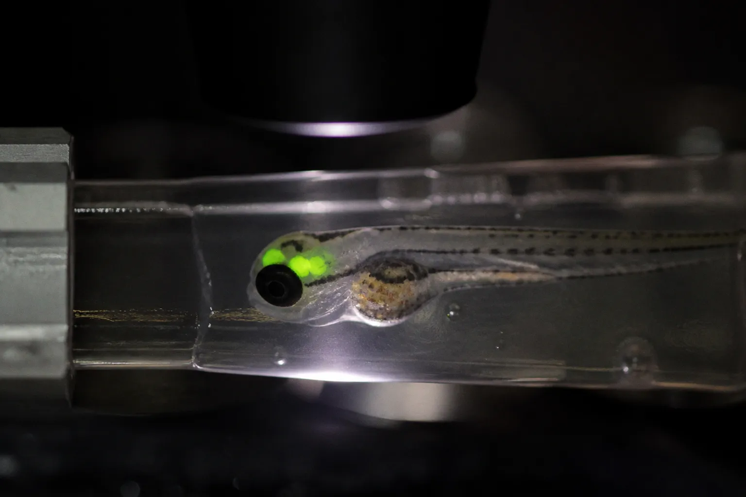
In an adult zebrafish olfactory bulb explant imaged with two-photon GCaMP6s, neurons were manually segmented after motion correction and the pre-stimulus baseline F0 was defined as the average fluorescence over ten seconds before stimulus onset. That window is long enough to average out brief spontaneous events, short enough that bleaching across a few trials is negligible, and well matched to the relatively slow kinetics of GCaMP6s in explant tissue. The choice makes sense in context: the preparation is stable, the stimulus timing is discrete, and the baseline is intended to represent a broad pre-stimulus state rather than the fluorescence in a narrowly defined respiratory phase.
The awake-mouse example requires more careful wording. Trials were acquired at roughly 30 Hz, with 400 frames per trial. The first 100 frames therefore span about 3.3 seconds, not one second. Those frames formed the available pre-odor period, but F0 was calculated from a one-second pre-odor baseline. That distinction matters. The recording contained a longer lead-in, while the normalization used a shorter portion of it. Treating “100 frames” and “one second” as interchangeable would make the timing look internally inconsistent and could lead someone reproducing the analysis to select the wrong samples.
A 2026 olfactory bulb study tightened the reference window further, defining F0 as the mean raw fluorescence over a 0.45-second period from 500 to 50 milliseconds before odor inhalation. Glomerular responses were then expressed as ΔF/F0, with responsiveness assessed relative to baseline variability using standard-deviation thresholds. This approach is useful when the event is locked to inhalation and the experiment is designed around a precise pre-event interval. It is less forgiving of spontaneous events inside the window, but it reduces the chance that slow changes in sniffing or illumination will be folded into the immediate pre-inhalation reference.
| Preparation | Baseline window used or illustrated | Why this scale |
|---|---|---|
| Adult zebrafish olfactory bulb explant, GCaMP6s, two-photon imaging | About 10 seconds before stimulus | A broad window can stabilize F0 in a relatively quiet explant and accommodate slow indicator kinetics |
| Awake mouse olfactory bulb, roughly 30 Hz, 400 frames per trial | The first 100 frames cover about 3.3 seconds; F0 was calculated from a 1-second pre-odor period | The longer recording lead-in provides context, while the shorter F0 window stays closer to odor onset in a spontaneously active preparation |
| Inhalation-locked olfactory bulb study | 0.45 seconds, from 500 to 50 milliseconds before inhalation | A narrowly defined pre-event interval aligns the reference to the respiratory event and limits slower drift |
The point is not that one of these windows is “correct.” The point is that the window has to be chosen for the kinetics of the indicator, the noise floor of the preparation, and the timing precision of the stimulus. A ten-second baseline in a spontaneously bursting awake preparation may include spontaneous calcium transients and other state changes, so its mean can sit above the fluorescence level immediately before the odor. That may be acceptable if the analysis is meant to describe a broader pre-stimulus state; it is a problem if the goal is to quantify the response relative to the moment just before inhalation.
The reverse problem is just as real. A 0.45-second baseline in an explant with slow kinetics may be dominated by whatever the cell happened to do during that narrow interval. If an event begins shortly before stimulus delivery, the “baseline” is already contaminated by the response. If the indicator has a slow decay from an earlier event, the pre-stimulus value is not a clean resting reference even when the trace looks visually quiet.
A useful way to choose the window is to ask what biological comparison the ΔF/F is meant to support:
- For trial-by-trial odor responses, stay close enough to stimulus onset that F0 reflects the same state as the response.
- For broad changes across a long recording, use a window or estimator that captures the local baseline without pretending every trial begins from an identical resting level.
- For inhalation-locked analysis, define the window relative to the respiratory event rather than only by an arbitrary frame count.
- For slow indicators, inspect whether the pre-stimulus period contains residual fluorescence from an earlier response.
- For awake recordings, examine spontaneous activity directly instead of assuming that a longer window automatically produces a better estimate.
There is also a practical distinction between the baseline window available in the acquisition and the baseline window used in the calculation. The camera may record several seconds before odor delivery to allow motion stabilization, timing checks, and quality control. That does not mean the entire lead-in must enter F0. Keeping the full lead-in visible is often valuable, but the normalization interval should be explicitly defined and reported.
Choose your baseline window the way you’d choose a frame around a portrait: tight enough to be honest about the resting face, wide enough that a single blink does not become the whole picture.
The baseline is not always a single average
A mean is convenient, but it is not automatically robust. One spontaneous event can pull the mean upward. A slow decline in fluorescence can make the early part of the window more influential than the late part. If the trace contains a brief motion artifact, the average may become an estimate of the artifact rather than of the tissue.
For that reason, it helps to plot the baseline interval and record more than its mean during method development. The median, standard deviation, minimum, and trend across the window can reveal whether F0 is being estimated from a stable segment or from a mixture of activity and drift. These diagnostics do not replace the chosen method, but they show whether the method is being asked to solve the wrong problem.
The same applies to trial averaging. If multiple odor presentations are aligned and averaged before baseline normalization, a response in one trial can alter the reference for another. In most cases, it is safer to define F0 at the trial level, after motion and background handling, and then average normalized traces. If the experiment instead requires a session-level baseline, that choice should be treated as part of the biological model, not as a harmless preprocessing shortcut.
Managing Photobleaching and Signal Drift in Long-Term Recordings
Baseline normalization and bleaching correction are not the same problem, even though both can bend a trace downward. Photobleaching is a loss of fluorescence caused by excitation and fluorophore chemistry. Baseline normalization is a decision about what counts as the reference fluorescence for a response. One describes the behavior of the signal during acquisition; the other describes how the signal is scaled for analysis.
You can have a clean pre-stimulus baseline in a heavily bleached preparation, and you can have a stable fluorophore whose baseline is defined badly. If the whole session fades gradually, each trial may still have a well-behaved local F0, but responses late in the recording will not be directly comparable with responses early in the recording unless the drift is addressed. Conversely, if the signal is stable but the pre-stimulus window contains spontaneous activity, applying a bleaching correction will not solve the real problem.
The zebrafish olfactory bulb work in the reference set handled photobleaching by attenuating excitation light to 1.5% of full intensity specifically to minimize fluorescence loss. The analysis then explicitly chose not to apply bleach correction, on the reasoning that correction could add noise and the remaining bleaching was small enough not to require it. That is a defensible position when bleaching has been measured or shown to be negligible. “No correction” is not the same as “we forgot correction”; it is a correction policy that should be supported by the behavior of control traces.
When the drift is not negligible, the awake-mouse workflow offers a different approach. The mean ROI fluorescence was concatenated across trials, the concatenated signal was detrended using a standard detrending function, and the data were reshaped back into trials before relative fluorescence change was calculated. The logic is sound when the dominant drift belongs to the session rather than to individual stimulus events. A session-level trend should be estimated from the session-level signal, not rediscovered independently in every short trial.
That order matters. If you detrend each trial separately, the algorithm can mistake a genuine slow response, an adaptation process, or a gradual recovery for an instrumental trend. If you detrend after ΔF/F, the denominator may already contain the drift you hoped to remove. Neither operation is universally wrong, but both make the underlying assumptions harder to see.
A few operational rules follow:
- If excitation power is modest, the preparation is stable, and the session is short, do not add detrending merely because it is available. A correction that is not needed can add variance and obscure genuine trial-to-trial differences.
- If the recording spans many minutes or many trials, inspect the mean fluorescence of stable reference ROIs and ask whether a session-level trend is present before choosing a correction model.
- Estimate a smooth drift from a signal that has not been contaminated by large stimulus-locked responses, or mask those periods when fitting the trend.
- Avoid fitting an aggressive polynomial or smooth curve that follows the response itself. The correction should remove a slow instrumental trend, not rewrite the biology.
- Keep the uncorrected trace. A corrected trace without its raw counterpart makes it difficult to tell whether the baseline fix improved the measurement or simply made it look cleaner.
- Do not use a rolling percentile baseline as a substitute for a photobleaching model. A percentile follows the distribution of fluorescence values; it does not know whether the fluorophore is being consumed by illumination.
The last point is particularly important in olfactory bulb recordings, where slow biological activity can look like drift. Odor exposure, changes in sniffing, spontaneous network events, and movement can all alter the fluorescence distribution over time. A method that tracks the lower tail of that distribution may absorb some of these changes into the baseline. That can be useful for a continuously active recording, but it is not evidence that photobleaching has been corrected.
Session drift versus trial drift
The distinction between session drift and trial drift is more than a technical detail. Session drift is often monotonic or slowly varying across the entire acquisition. Trial drift may reflect incomplete recovery from an earlier odor, a change in respiration, a shift in focus, or a response-dependent change in the fluorescence distribution. These causes can produce similar-looking traces while requiring different handling.
A simple diagnostic is to compare several quantities across trial number:
1. The raw mean fluorescence in the ROI.
2. The baseline fluorescence before each odor.
3. The peak response after normalization.
4. A reference region that should not respond to the odor.
5. Motion metrics or registration quality.
If raw fluorescence declines while the reference region behaves similarly, photobleaching or illumination drift becomes plausible. If only one glomerulus changes and the change follows repeated odor presentation, adaptation or biology is more plausible. If baseline shifts occur at the same time as motion changes, registration or tissue movement may be the dominant problem.
This is why a “fast baseline fix” should not begin with a formula. It should begin with a trace that has been separated into acquisition behavior, tissue behavior, and analysis behavior as far as the data allow.
Advanced Baseline Estimation: Kernel-Density and Percentile Approaches
For long or continuously active recordings, a static pre-stimulus window is fragile. The animal breathes, the indicator drifts, the focus may shift, and the cell or glomerulus rarely sits politely at rest. Two useful families of methods are running-percentile baselines and kernel-density baselines. Both can be effective, but both encode assumptions about what the fluorescence distribution means.
Running percentiles
The running-percentile approach estimates a local baseline from a moving section of the trace. CaImAn documentation provides a familiar example: use a long window of around 100 seconds and estimate the 10th percentile within that window as the local baseline. Values between window positions can be interpolated to produce a smoother baseline and reduce the computational burden of calculating the estimate at every frame.
The appeal is obvious. A percentile is less sensitive than a mean to isolated calcium transients, and the moving window allows the baseline to follow slow changes in illumination or indicator expression. For sparse activity, the lower tail of the fluorescence distribution can be a reasonable approximation of the non-event state.
But the method does not identify rest by magic. It assumes that the lower portion of the observed fluorescence distribution contains enough periods without meaningful activity. If the cell is active for most of the window, the tenth percentile may represent a low-activity state rather than a true baseline. If neuropil contamination is strong, its fluctuations may define the lower tail. If the recording contains a prolonged response, the percentile can rise and gradually normalize the response away.
The window length therefore has a biological interpretation. A very long window is stable but slow to adapt. A short window follows changes rapidly but is more vulnerable to local activity and noise. The right choice depends on how quickly the baseline can plausibly change and how frequently the tissue can plausibly return to a low-activity state.
Kernel-density estimation
The kernel-density approach takes a different route. In the real-time two-photon pipeline that established this method, the preceding 2,000 frames were divided into 100 bins of 20 frames. A mean was computed for each bin, producing a distribution of 100 local averages. The baseline was then estimated from the peak of the kernel-density distribution over those averages.
This method uses the most common local fluorescence state as the reference. That can be more stable than selecting a single low percentile when the trace is noisy, because each bin contributes an average rather than an individual frame. Across the noise and activity levels tested, the kernel-density method produced a consistent baseline estimate.
Its central assumption is also its limitation: rest, or something close to rest, must be the most frequently visited state. If the cell spends most of the recording in an active state, the density peak can follow that active state. In a preparation with strong rhythmic activity, the peak may reflect the most common phase or amplitude of the rhythm rather than a fluorescence floor. Kernel density can make the estimate look statistically sophisticated while still being biologically misassigned.
| Method | Best suited to | Main assumption | What to inspect |
|---|---|---|---|
| Pre-stimulus window | Discrete odor puffs and relatively quiet preparations | The selected pre-event interval represents the relevant resting state | Spontaneous events, residual indicator decay, and local drift |
| Running percentile, such as the 10th percentile over about 100 seconds | Long traces with slow drift and sparse activity | The lower tail contains enough low-activity periods | Whether continuous or prolonged activity has lifted the percentile floor |
| Kernel density over binned history | Real-time pipelines and noisy, continuously sampled cells | The most common local fluorescence state is close to baseline | Whether the density peak corresponds to rest, rhythmic activity, or a persistent response |
The right baseline is the one that does the least violence to the biology you are actually trying to see.
How to compare estimators without choosing by appearance
A baseline can make a trace look cleaner while making the measurement less faithful. Comparing methods by visual smoothness is therefore a poor validation strategy. Instead, apply candidate estimators to the same raw ROI trace and compare what each one does to several known or controlled features:
- Does the baseline remain stable during a no-odor period?
- Does it move during a sustained odor response?
- Does it follow an obvious illumination trend without following individual calcium events?
- Does it produce comparable response amplitudes across repeated trials?
- Does it preserve the timing of onset and recovery?
- Does it behave similarly in responsive and nonresponsive glomeruli?
For a zebrafish olfactory bulb imaging analysis, this comparison is especially useful when the tissue is continuously active or when the recording is long enough for illumination and focus to change. A fixed ten-second F0 may be entirely adequate for one experiment and inappropriate for another recorded with the same indicator. The method should follow the recording regime, not the label attached to the preparation.
It is also worth separating the baseline estimate from the response metric. A peak ΔF/F, integrated response, response latency, and area under the curve can react differently to the same baseline error. A baseline that is slightly too high compresses positive responses; a baseline that is too low inflates them. A drifting baseline can distort integrated response even when the peak appears reasonable. If the biological conclusion depends on more than one metric, the baseline should be tested against all of them.
Distinguishing Background Subtraction from Baseline Normalization
The most common conceptual error in olfactory bulb image analysis is treating background subtraction and ΔF/F calculation as one operation. They are not.
Background subtraction removes fluorescence that does not belong to the signal of interest: camera offset, out-of-focus light, diffuse neuropil, and other non-cellular or non-glomerular contributions. Baseline normalization then sets the resting cellular or glomerular fluorescence against which a response is measured. The first changes the signal being analyzed. The second scales that signal over time.
A quantitative fluorescence imaging study using olfactory bulb slices reported that inaccurate background subtraction can produce errors reaching 100% in estimates of resting calcium and calcium dynamics. That is large enough to overwhelm typical ΔF/F responses and makes the distinction impossible to ignore. If the background estimate is wrong, a careful F0 calculation can still normalize the wrong fluorescence.
The order of operations should therefore be explicit. A defensible workflow is:
1. Register the imaging session. Correct motion across the full recording before extracting the final ROI trace. If the ROI moves relative to the tissue, the fluorescence changes can look like calcium events.
2. Inspect and estimate background. Use a background region or neuropil estimate appropriate to the preparation, and document how that region was selected.
3. Subtract the estimated background. Apply the subtraction consistently across frames and trials. A neuropil coefficient near 0.7 is often used in calcium imaging workflows, but there is no universal coefficient established specifically for every olfactory bulb preparation.
4. Define F0. Choose the pre-stimulus, percentile, kernel-density, or other estimator after background handling and drift decisions have been made.
5. Calculate ΔF/F. Keep the formula and the exact reference interval recorded for each dataset.
6. Deconvolve only if needed. If the goal is to infer event timing or spiking from the calcium trace, perform deconvolution on the processed ΔF/F signal and state that the result is an inference, not a direct spike measurement.
The precise implementation can vary, but collapsing all six steps into “baseline correction” makes errors difficult to locate. If a response is unexpectedly large, the problem may be ROI contamination rather than F0. If a response disappears after normalization, the estimator may be tracking the response. If the raw trace is stable but ΔF/F drifts, the denominator may be changing even though the numerator is not.
Neuropil is not merely background
In the olfactory bulb, neuropil deserves special attention because glomeruli are dense synaptic structures rather than isolated cell bodies. A glomerular ROI can contain signal from nearby axons, dendrites, processes, and diffuse fluorescence. Subtracting a nearby region can reduce this contamination, but the region itself may carry odor-evoked activity. The background is therefore not necessarily an inert black level.
A useful background region should be close enough to experience similar illumination and optical conditions, but not so close that it simply duplicates the response of the target glomerulus. That balance is preparation-specific. The selected region, coefficient, and whether the background is static or time-varying should be retained in the analysis record.
Subtracting too much can be as damaging as subtracting too little. Overcorrection can create negative dips, suppress genuine broad responses, and amplify noise when the background estimate is itself variable. Under-correction leaves shared activity in the trace and can make neighboring glomeruli appear more correlated than they are. The right question is not whether a subtraction coefficient is familiar; it is whether the resulting trace behaves plausibly in controls and across ROIs.
CaImAn documentation notes that ΔF/F extraction can be performed before deconvolution and that this can reduce the impact of drifting baselines. That is useful, but it does not remove the need for honest background handling. Deconvolution cannot recover information that was already mixed with unmodeled neuropil activity, and a percentile estimator cannot tell whether a low-frequency component came from the cell, the neuropil, or the microscope.
Validation Strategies for Reliable Glomerular Response Quantification
No baseline method is self-validating. The 2026 olfactory bulb study assessed responsiveness relative to baseline variability using standard-deviation thresholds, a common operational approach: a response counts if its peak rises by some multiple of the standard deviation above the F0 window. This provides a useful guardrail, but it is not independent of the baseline choice. If the baseline window contains a transient, its standard deviation rises and the responsiveness threshold rises with it. If the window is too short, the estimate of variability becomes unstable.
A threshold should therefore be treated as one piece of evidence rather than as proof that the baseline is correct. Before trusting a response value, inspect:
- the raw fluorescence trace beside the ΔF/F trace, using the same time axis;
- the F0 window marked on both traces;
- stimulus onset, odor duration, and, where relevant, inhalation timing;
- a no-odor or vehicle control processed through the identical pipeline;
- an ROI or glomerulus expected not to respond under the same conditions;
- motion-correction quality and any frame periods excluded from analysis;
- the behavior of the baseline estimator during the response and recovery periods;
- repeated presentations of the same odor, including the order in which they occurred.
The raw trace should remain visible because normalization can conceal the scale of the underlying problem. A small raw fluctuation divided by a very low F0 can produce a large ΔF/F. Conversely, a real response can look modest if the denominator includes residual activity from the preceding trial. Neither conclusion can be evaluated from the normalized trace alone.
Controls that test the pipeline rather than the biology
A no-odor trial is not only a control for false biological responses. It is also a test of motion, illumination stability, and the baseline estimator. If the no-odor trace shows a slow response-shaped deflection, the pipeline may be converting drift into biology. If the vehicle produces a transient, the delivery system or fluid movement may be part of the signal.
Repeated odor trials test a different property: reproducibility. A glomerulus need not produce identical amplitudes on every trial, especially in an awake animal, but the baseline should not create a systematic pattern that is absent from the raw fluorescence. If normalized responses grow while raw fluorescence remains stable, the denominator may be falling. If normalized responses shrink while the raw peak is unchanged, the baseline may be rising.
A neighboring or nonresponsive ROI can reveal shared artifacts. When several ROIs move together during a frame shift, the event is probably not a glomerulus-specific calcium response. When all ROIs decline together across the session, illumination or focus deserves attention. When only a single ROI changes in a way that aligns with its anatomy and stimulus selectivity, the biological interpretation becomes stronger — provided the raw trace supports it.
A compact validation pass
Before extracting a final response table, run the same inspection on a small set of representative traces:
1. Choose a strongly responsive glomerulus, a weakly responsive glomerulus, and a presumed nonresponsive region.
2. Display raw fluorescence, background estimate, corrected fluorescence, F0, and ΔF/F together.
3. Mark the baseline and stimulus windows explicitly.
4. Compare the fixed-window result with at least one alternative estimator when the recording is long or active.
5. Check whether the response classification changes because of the estimator rather than because of the data.
6. Review control trials and motion metrics before deciding which method is defensible.
This is not a demand for manual inspection of every frame. It is a demand that the analysis be auditable. A baseline algorithm can be automated; its assumptions cannot be outsourced to the software.
If a control trial produces a response, the baseline is doing work it should not be doing. If the same glomerulus drifts across trials under identical stimulus conditions, either bleaching correction is missing, the preparation is changing, or the estimator is chasing activity. If only the ΔF/F drifts while the corrected raw signal does not, inspect the denominator first. If both drift together, return to motion, illumination, and background.
ΔF/F is a ratio, not a measurement. The number is only as quiet as the floor beneath it.
Closing Principle
The fastest baseline fix in olfactory bulb calcium imaging is not a single number. It is a deliberate stack of small choices, each matched to a specific feature of the preparation: a temporal window that respects indicator kinetics, a reference interval that is stated in both frames and time, a bleaching correction applied only when bleaching is actually present, a baseline estimator whose assumptions fit the activity pattern, and a background subtraction performed before normalization rather than hidden inside it.
For zebrafish olfactory bulb imaging analysis, a ten-second pre-stimulus average may be a sensible choice in a stable explant with slow GCaMP6s kinetics. In an awake mouse recording acquired at roughly 30 Hz, the first 100 frames represent about 3.3 seconds of pre-odor data, while the analyzed F0 may still be the one-second interval immediately before odor onset. In an inhalation-locked experiment, a 0.45-second window from 500 to 50 milliseconds before inhalation may be the more meaningful reference. These are not contradictions. They are different answers to different experimental questions.
Do not treat a long baseline as automatically more reliable. It may include spontaneous activity. Do not treat a short baseline as automatically more precise. It may capture a transient or residual indicator signal. Do not detrend because a curve looks untidy. First establish that the drift is real, then choose a correction that cannot erase the biology under study. Do not let background subtraction disappear into a generic preprocessing label. The neuropil estimate, subtraction coefficient, and normalization window all shape the final calcium signal.
Choose the window to match the brain state. Correct drift only when the data show drift. Keep background subtraction and baseline normalization as separate steps. Compare the corrected trace with the raw fluorescence, not with a more attractive corrected trace. Inspect controls before extracting response amplitudes.
That is the floor. Everything luminous in the trace is built on top of it.