Zebrafish olfactory mapping: from preparation to final data
You've pulled the fish out of the tank, you've pipetted what should be a perfect bolus of indicator into the naris, you've waited your five minutes, and now your calcium trace looks like someone is fanning the dish with a magazine.
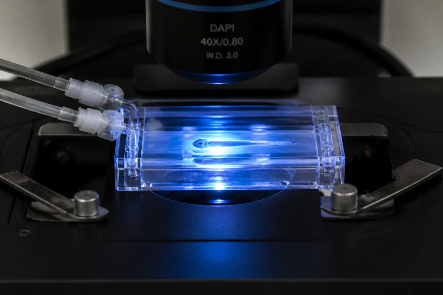
The First Five Minutes: Why Your Map Looks Like Static
The glomeruli smear into each other, the boundaries melt before you can register them, and every sniff response arrives half a second too late. We have all been there, and it is almost never the camera. It is almost always what happened in the first five minutes of prep.
That is the part of zebrafish olfactory bulb mapping that nobody warns you about — the prep is the protocol. Get the indicator loading right, get the explant cold and clean, get the odor pulse honest, and the rest of the workflow becomes a pleasure instead of a punishment. So let's walk through the whole pipeline, bench to glomerulus, and fix the six places where your signal usually dies before it ever reaches the screen.
A clean glomerular map starts in the fish tank, not on the optical table — every step you rush in the first ten minutes shows up as noise in the last ten frames.
Loading Calcium Indicators Into OSNs
We have tried about a dozen ways to get calcium reporters into zebrafish olfactory sensory neurons, and the only one that gives a reliable, broad-spectrum label without crushing viability is the dye-into-naris protocol. The biology is on your side here: olfactory sensory neurons sit just behind the naris in a thin, accessible epithelial sheet, and if you give them a brief bolus of membrane-permeable dextran-conjugated indicator under a touch of detergent, they take it up cleanly and traffic it down their axons to the bulb within the hour.
Here is the prep we run every single week:
1. Anesthetize the adult zebrafish in 0.01% MS-222 until gill movement slows and the tail flick stops on handling. You want a fish that is fully unresponsive, not a fish that twitches when you touch the flank.
2. Prepare your indicator working solution fresh: 6–8% Calcium Green-1 dextran (10 kDa) dissolved in 3 mM NaCl, with 0.1% Triton X-100 added at the bench. The Triton is not optional — it is the difference between a uniformly labeled sheet of OSNs and a dim, patchy one that will haunt your baseline fluorescence for the rest of the day.
3. Lay the fish on a damp sponge under a dissecting scope, dorsal side up, head tilted slightly forward. Use a fine-mouth pipette to deliver ~1 μl of the dye solution directly into each naris. Slow delivery — let the bolus sit in the cup of the naris rather than running off the head.
4. Hold the fish in a humid chamber for 5 minutes. Do not let the gills dry out. Do not let the dye run backward into the opercular cavity.
5. Return the fish to system water for a 30–45 minute recovery window. The OSNs need this window to traffic the dye into their axons and into their glomerular terminals. Skip it and you will be looking at epithelial signal that never made it to the bulb.
What if your fish is small, juvenile, or one of those skinny transgenic lines that always seem to be the most interesting? Drop the dye volume to ~0.5 μl per naris and use a finer-bore pipette. We have found that pushing above 1 μl in fish under 30 mm standard length just washes the bolus straight past the olfactory epithelium and into the opercular cavity, and you lose most of your loading efficiency. What if you are working with a calcium indicator that is not dextran-conjugated and is membrane-permeable on its own? Skip the Triton. The detergent is there to permeabilize the apical membrane just enough for the dextran to slip through, and if your dye crosses on its own, the Triton becomes a viability tax rather than a help.
Treat the recovery window as part of the protocol, not as downtime — the dye is still moving while the fish sits in the tank.
Pulling the Brain-Nose Explant Without Crushing It
This is the step where most labs lose their prep, and it is the step that takes the longest to learn. The ex vivo brain-nose explant is gorgeous when it works — both olfactory bulbs sit ventral and exposed, the nasal epithelium stays attached via the intact olfactory nerve, and the whole preparation responds to odors for hours. The trick is that you are doing microsurgery on a soft, cold, slippery brain, and the only thing holding the bulbs in anatomical position is connective tissue you cannot see until you have already torn it.
Here is the cleanest version we have found:
1. After recovery, re-anesthetize the fish in 0.01% MS-222 and transfer it to a dish of ice-cold artificial cerebrospinal fluid (ACSF) pre-bubbled with carbogen. The 4°C chill is not cruelty — it slows metabolism so the brain survives the dissection without firing off a stress response that will drown your first stimulus.
2. Decapitate the fish just behind the operculum with a fresh razor blade, in the ACSF bath, so the head never touches air. We do this under the scope so we can confirm the cut is clean.
3. Under higher magnification, remove the eyes, the jaws, and the thin bones overlying the ventral forebrain. The olfactory bulbs live on the ventral surface, anterior to the telencephalon, and they look slightly pinker than the surrounding tissue once the bone is cleared.
4. Carefully peel the ventral skin and bone away in one continuous motion, keeping the olfactory nerve intact between the bulbs and the nasal cavity. If you see the nerve stretching, you are pulling too hard — back off and clear more bone laterally before you try again.
5. Pin the explant ventral side up in a recording chamber perfused with oxygenated ACSF at room temperature (~22°C), using a weighted harp grid rather than sharp pins.
| Step | What goes wrong | How to fix it |
|---|---|---|
| Chilling | Brain warms before pinning | Keep the dish on ice; work in 90-second bursts |
| Bone removal | Bulb gets nicked by forceps | Use fine-tip iridectomy scissors; clear bone in layers |
| Olfactory nerve | Nerve snaps, bulb detaches | Stop pulling; clear more bone laterally first |
| Pinning | Explant rolls or floats | Use a weighted harp grid; never pierce the bulb itself |
The explant should sit flat, with both bulbs visible from the ventral view, and the nasal cavity still connected by the olfactory nerve. If your bulbs are curling or rolling in the chamber, your perfusion is too aggressive — drop the flow rate to 1–2 ml/min and let the chamber equilibrate before imaging.
Delivering an Odor Pulse That Actually Means Something
You can have the cleanest explant in the building and still get a junk trace if your odor delivery is sloppy. The zebrafish olfactory bulb responds on the timescale of tens of milliseconds, and if your stimulus takes 600 ms to reach peak concentration at the naris, you have already lost the first third of the response to convolution with your own delivery artifact. The glomerulus knows the odor arrived; your data does not.
We use a constant carrier stream of clean ACSF or charcoal-filtered air directed at the naris through a small-diameter needle, with a pneumatic HPLC injection valve that switches the carrier over to odorant-saturated solution for a defined pulse window. This setup gives you a square-ish stimulus that hits maximum concentration in ~600 ms and persists for ~2.4 seconds before the valve flips back to clean carrier.
| Parameter | Typical value | Why it matters |
|---|---|---|
| Carrier flow | 1–2 ml/min | Steady baseline; prevents mechano artifacts at the naris |
| Valve switching time | <50 ms | The sharper the edge, the cleaner your onset kinetics |
| Rise time to peak | ~600 ms | Defines the temporal resolution of your chemotopic map |
| Pulse duration | 2.4 s | Long enough to capture adaptation, short enough to avoid desensitization |
| Odorant concentration | 10–40 μM | Standard across amino acid and bile acid panels |
What if you are working with a hydrophobic odorant that does not dissolve cleanly into your aqueous carrier? Pre-dilute in DMSO to a 1000× stock, then dilute that stock 1:1000 into your carrier stream at the bench. Final DMSO concentration should stay below 0.1% — above that, you start seeing vehicle-only responses in your control traces. What if your odor pulse is inconsistent run-to-run? Check the valve rotor for wear; the rotor seals are the part that fails most often in pneumatic injection valves, and the failure mode is a slow leak that dilutes your stimulus rather than blocking it. Replace the rotor and your run-to-run variability collapses.
Wide-Field Imaging and Finding Your 140 Glomeruli
Now we get to the part that looks like science — and the part where most people reach for a two-photon microscope that they do not actually need. Wide-field calcium imaging of the zebrafish olfactory bulb is not a compromise. For the chemotopic maps we want to build, it is the right tool, and it has been the right tool since the early optical mapping work in this system.
We use a sensitive CCD camera binned to 128×128 or 170×170 pixels, with frame rates between 2 and 20 Hz depending on what we are asking. The binning is not laziness — it gives you enough photons per glomerulus per frame to push your signal-to-noise above 5:1, which is the threshold below which temporal deconvolution starts hallucinating spikes and your tuning curves become unreliable. Two-photon gives you optical sectioning, but for a ventral-surface preparation that already sits in a thin optical plane, that sectioning is buying you depth resolution you do not need.
The zebrafish olfactory bulb contains approximately 140 glomeruli, of which about 27 are easily recognizable landmarks you can use to register across fish. The chemotopic organization is consistent enough to anchor on:
| Bulb region | Predominant ligands | Practical notes |
|---|---|---|
| Lateral cluster | Amino acids | High signal-to-noise; ideal for tuning curves |
| Medial cluster | Bile acids | Smaller glomeruli; more cross-fish variability |
| Dorsal cap | Pheromones, alarm cues | Sparse; needs averaging across trials |
When you align your first map to a reference atlas, register on the 27 recognizable glomeruli first and let the interpolation fill in the rest. Do not try to assign all 140 by eye — you will over-fit to your own prep and lose the chemotopic structure that is the actually interesting signal.
What if your glomerular boundaries look fuzzy? Drop your binning to 256×256 for a single test fish and see whether spatial resolution was the bottleneck, or whether the boundaries are smeared by motion artifact. In our experience, it is motion nine times out of ten — the explant is alive, the cilia are still beating, and every frame is a tiny translation away from the previous one. Rigid motion correction with a sub-pixel registration algorithm will fix 90% of the fuzz. If motion correction does not help, your indicator loading was uneven, and you need to go back to step one.
From Calcium Signal to Spike Train: Temporal Deconvolution
This is where most labs stop, and it is a shame, because the raw calcium signal is a low-pass filtered, laggy, noisy approximation of the underlying spiking. If you want to know whether two glomeruli are firing at the same time or whether one is leading the other by 50 ms, you need to deconvolve.
Temporally deconvolved Ca²⁺ imaging (TDCa imaging) reconstructs changes in firing rates from somatic calcium signals by applying a kernel that represents a unitary calcium transient — the stereotyped rise and decay that a single spike produces in your particular indicator under your particular loading conditions. Convolving this kernel with an estimated spike train should reproduce your measured calcium trace; deconvolution is the inverse operation: given the measured trace and the kernel, what spike train is most likely to have produced it?
The practical effect is that you push your effective temporal resolution from the frame rate of your camera up to the underlying biological timescale. A 5 Hz acquisition becomes, after deconvolution, something that can resolve 50–100 ms events. The onset latency of glomerular responses, the relative timing of lateral versus medial cluster activation, the duration of the sniff-locked burst — all of these become quantifiable after deconvolution, and they were buried in your raw trace before.
Temporal deconvolution is the difference between knowing that two glomeruli responded and knowing which one fired first.
What if your deconvolved trace looks too spiky, with every noise fluctuation becoming a "spike"? Your kernel is too sharp for the noise floor of your data. Smooth the kernel by 20–30% and re-run. What if your deconvolved trace looks identical to your raw calcium trace, and you have gained nothing? Your kernel is too smooth for your indicator, or your frame rate is too low for the deconvolution to add information. Push the frame rate up to 10–20 Hz before re-deconvolving, and re-estimate the kernel from your own data rather than borrowing one from a paper.
Mitral Cells, Multi-Glomerular Integration, and the Interhemispheric Trick
Now the part that makes zebrafish olfaction genuinely weird compared to mammals, and the part that will reshape how you read every map you just built. Mitral cells in zebrafish do not project to a single glomerulus. A single zebrafish mitral cell sends several dendrites out to multiple glomeruli, which means it is sampling input from several different odorant receptors simultaneously. The chemotopic map you built is the input space; the mitral cell layer is where that input space is being mixed, decorrelated, and recombined before the signal ever reaches the telencephalon.
This changes how you read your chemotopic map. If two glomeruli are firing strongly in your data, you cannot assume that downstream neurons are reading them independently — they may be pooled by the same output mitral cell. The classic "one glomerulus, one receptor, one mitral cell" rule from mammalian olfactory bulb anatomy does not hold in zebrafish. It is a multi-glomerular, integrative circuit at the very first step of central processing, and your analysis has to reflect that.
And there is one more piece of the wiring that will catch you off guard the first time you see it in your own data: there are direct interhemispheric projections between the left and right olfactory bulbs. Axons from mitral cells in one hemisphere cross over and terminate in glomeruli in the contralateral hemisphere, and the targeting is not random — contralateral mitral cell axons connect similarly tuned glomeruli across the two hemispheres. The functional consequence is that an odor pulse delivered to one naris modulates activity in the contralateral bulb, and the modulation is chemotopically organized. We do not yet know the exact molecular guidance cues that direct this targeting, but the wiring is there in every adult fish you prep.
What does that mean for your map? It means the left-bulb map and the right-bulb map are not independent replicates of each other — they are coupled. If you image one bulb and treat it as a closed preparation, you are missing the contralateral modulation entirely. The cleanest experiments image both bulbs simultaneously, register them to a common atlas, and analyze the cross-hemisphere correlation structure as part of the same dataset rather than as a follow-up.
Bringing It All Together
Zebrafish olfactory bulb mapping is six protocols glued together: a dye loading that respects OSN biology, a dissection that keeps the explant alive, an odor delivery that hits hard and ends clean, a wide-field imaging setup with the right binning, a temporal deconvolution that lifts your signal out of the calcium lag, and an analysis layer that knows mitral cells integrate across glomeruli and that the two hemispheres talk to each other through chemotopically organized projections.
Each step has a failure mode that is easy to diagnose once you have seen it, and almost impossible to diagnose if you have not. That is why we walk new lab members through all six in their first two weeks — not because any single step is hard, but because the failure modes compound. A noisy dye load becomes a fuzzy glomerular boundary becomes a meaningless deconvolution becomes a tuning curve that does not tune. Fix the prep, and the rest of the pipeline runs itself.
So pull a fresh fish, load your indicator with the Triton where it belongs, give it the recovery window you would want for yourself, pull the explant cold and clean, build your odor pulse honest, image wide-field with the right binning, deconvolve with a kernel that fits your indicator, and remember that one glomerulus is never the whole story. The map you build will be cleaner, the timing will be sharper, and you will finally stop blaming the camera.